Exploring Movie Trends (EDA)

ROI

GGPLOT

data wrangling

Published

31 August 2023

Set up

library(kableExtra)
library(tidyverse)
library(tvthemes)
library(ggthemes)
library(scales)
library(magrittr)

out_new<-vroom::vroom("movies.csv")
out_new |> 
  head(10) |> 
  kable(table.attr = "style = \"color: black;\"") |> 
  kable_styling(fixed_thead = T) |> 
  scroll_box(height = "400px")

...1	release_date	movie	production_budget	domestic_gross	worldwide_gross	distributor	mpaa_rating	genre
1	6/22/2007	Evan Almighty	1.75e+08	100289690	174131329	Universal	PG	Comedy
2	7/28/1995	Waterworld	1.75e+08	88246220	264246220	Universal	PG-13	Action
3	5/12/2017	King Arthur: Legend of the Sword	1.75e+08	39175066	139950708	Warner Bros.	PG-13	Adventure
4	12/25/2013	47 Ronin	1.75e+08	38362475	151716815	Universal	PG-13	Action
5	6/22/2018	Jurassic World: Fallen Kingdom	1.70e+08	416769345	1304866322	Universal	PG-13	Action
6	8/1/2014	Guardians of the Galaxy	1.70e+08	333172112	771051335	Walt Disney	PG-13	Action
7	5/7/2010	Iron Man 2	1.70e+08	312433331	621156389	Paramount Pictures	PG-13	Action
8	4/4/2014	Captain America: The Winter Soldier	1.70e+08	259746958	714401889	Walt Disney	PG-13	Action
9	7/11/2014	Dawn of the Planet of the Apes	1.70e+08	208545589	710644566	20th Century Fox	PG-13	Adventure
10	11/10/2004	The Polar Express	1.70e+08	186493587	310634169	Warner Bros.	G	Adventure

first things first ::

what variables do we have?

names(out_new)
#> [1] "...1"              "release_date"      "movie"            
#> [4] "production_budget" "domestic_gross"    "worldwide_gross"  
#> [7] "distributor"       "mpaa_rating"       "genre"

secondly ,what are the datatypes that we have?

map_dfr(out_new,class)
#> # A tibble: 1 × 9
#>   ...1    release_date movie    production_budget domestic_gross worldwide_gross
#>   <chr>   <chr>        <chr>    <chr>             <chr>          <chr>          
#> 1 numeric character    charact… numeric           numeric        numeric        
#> # ℹ 3 more variables: distributor <chr>, mpaa_rating <chr>, genre <chr>

This data was featured in the FiveThirtyEight article,“Scary Movies Are The Best Investment In Hollywood”.

Now let`s describe the dataset

Header	Description
`release_date`	month-day-year
`movie`	Movie title
`production_budget`	Money spent to create the film
`domestic_gross`	Gross revenue from USA
`worldwide_gross`	Gross worldwide revenue
`distributor`	The distribution company
`mpaa_rating`	Appropriate age rating by the US-based rating agency
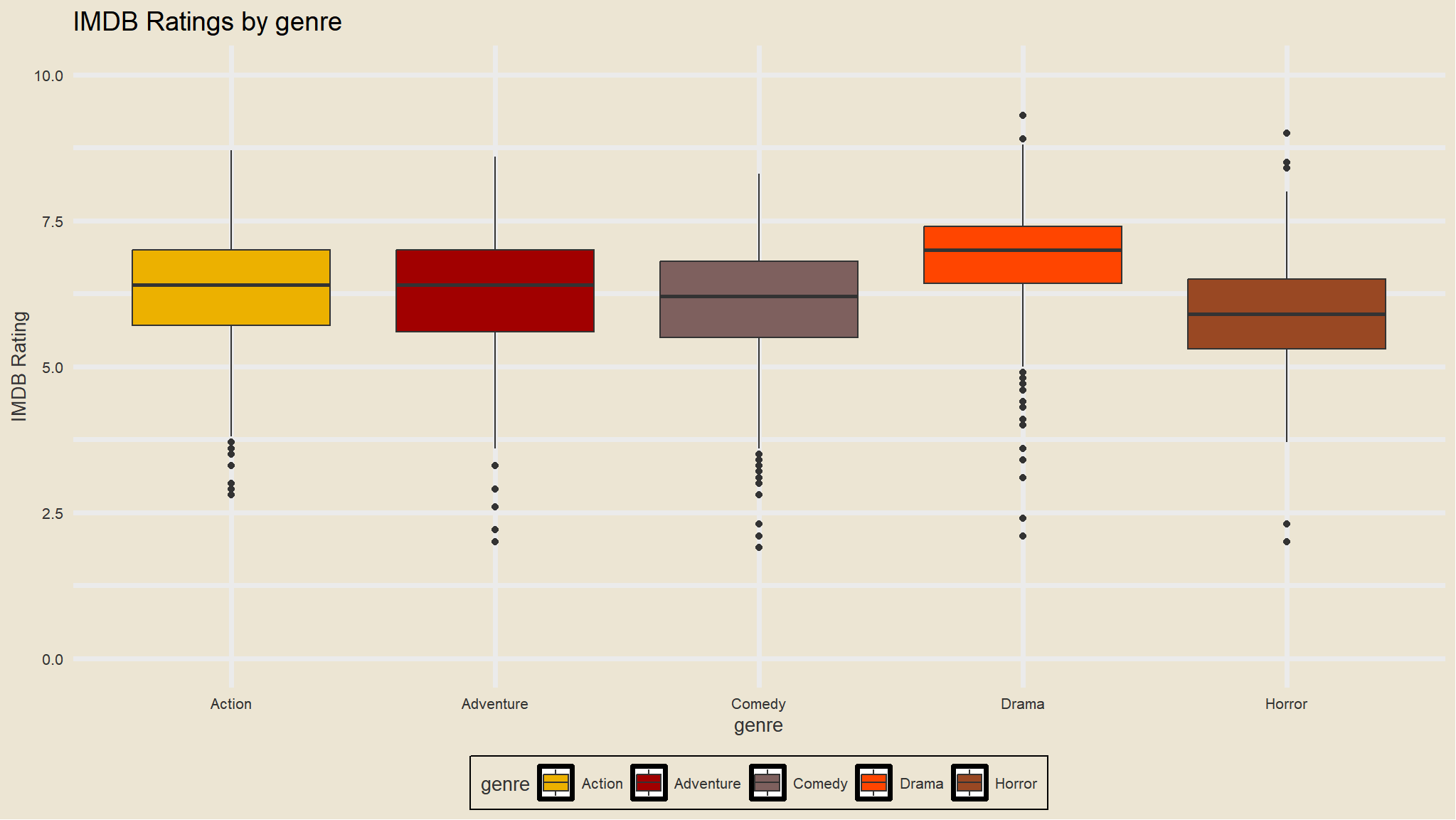
`genre`	Film category

let’s do some touches on the dataset

Get rid of the blank X1 Variable.
Change release date into an actual date.
change character variables to factors
Calculate the return on investment as the worldwide_gross/production_budget.
Calculate the percentage of total gross as domestic revenue.
Get the year, month, and day out of the release date.
Remove rows where the revenue is $0 (unreleased movies, or data integrity problems), and remove rows missing information about the distributor. Go ahead and remove any data where the rating is unavailable also.

…. but before that lets skim a bit!

out_new |> skimr::skim()

Data summary
Name	out_new
Number of rows	3401
Number of columns	9
_______________________
Column type frequency:
character	5
numeric	4
________________________
Group variables	None

Variable type: character

skim_variable	n_missing	complete_rate	min	max	n_unique
release_date	0	1.00	8	10	1768
movie	0	1.00	1	35	3400
distributor	48	0.99	3	22	201
mpaa_rating	137	0.96	1	5	4
genre	0	1.00	5	9	5

Variable type: numeric

skim_variable	complete_rate	mean	sd	p0	p25	p50	p75	p100	hist
…1	1	1701	981.93	1	851	1701	2551	3401	▇▇▇▇▇
production_budget	1	33284743	34892390.59	250000	9000000	20000000	45000000	175000000	▇▂▁▁▁
domestic_gross	1	45421793	58825660.56	0	6118683	25533818	60323786	474544677	▇▁▁▁▁
worldwide_gross	1	94115117	140918241.82	0	10618813	40159017	117615211	1304866322	▇▁▁▁▁

mov <- out_new |>
  select(-1) |>
  mutate(release_date = mdy(release_date)) |> #mdy is the setup of the date variable
  mutate_if(is.character,as.factor) |> 
  mutate(roi = worldwide_gross / production_budget) |>
  mutate(pct_domestic = domestic_gross / worldwide_gross) |>
  mutate(year = year(release_date)) |> 
  mutate(month = month(release_date)) |> 
  mutate(day = as.factor(wday(release_date))) |> 
  arrange(desc(release_date)) |>
  filter(worldwide_gross > 0) |>
  filter(!is.na(distributor)) |>
  filter(!is.na(mpaa_rating))
mov
#> # A tibble: 3,202 × 13
#>    release_date movie           production_budget domestic_gross worldwide_gross
#>    <date>       <fct>                       <dbl>          <dbl>           <dbl>
#>  1 2018-10-12   First Man                60000000       30000050        55500050
#>  2 2018-10-12   Goosebumps 2: …          35000000       28804812        39904812
#>  3 2018-10-05   Venom                   100000000      171125095       461825095
#>  4 2018-10-05   A Star is Born           36000000      126181246       200881246
#>  5 2018-09-28   Smallfoot                80000000       66361035       137161035
#>  6 2018-09-28   Night School             29000000       66906825        84406825
#>  7 2018-09-28   Hell Fest                 5500000       10751601        12527795
#>  8 2018-09-14   The Predator             88000000       50787159       127987159
#>  9 2018-09-14   White Boy Rick           30000000       23851700        23851700
#> 10 2018-08-17   Mile 22                  35000000       36108758        64708758
#> # ℹ 3,192 more rows
#> # ℹ 8 more variables: distributor <fct>, mpaa_rating <fct>, genre <fct>,
#> #   roi <dbl>, pct_domestic <dbl>, year <dbl>, month <dbl>, day <fct>

fair enough , the date variable looks pretty good now !
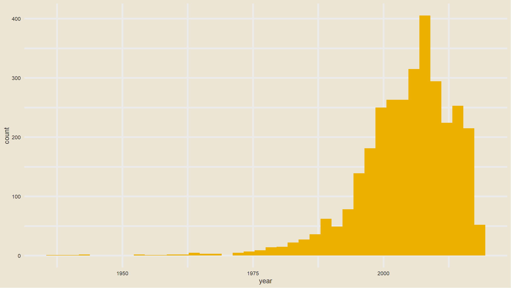
let us look at the distribution of the year variable

ggplot(mov, aes(year)) + 
  geom_histogram(bins=40, fill=avatar_pal()(1))+
  theme_avatar()

There doesn’t appear to be much documented before 1975, so let’s restrict (read: filter) the dataset to movies made since 1975. Also, we’re going to be doing some analyses by year, and the data for 2018 is still incomplete, let’s remove all of 2018. Let’s get anything produced in 1975 and after (>=1975) but before 2018.

filter and remove the years described above

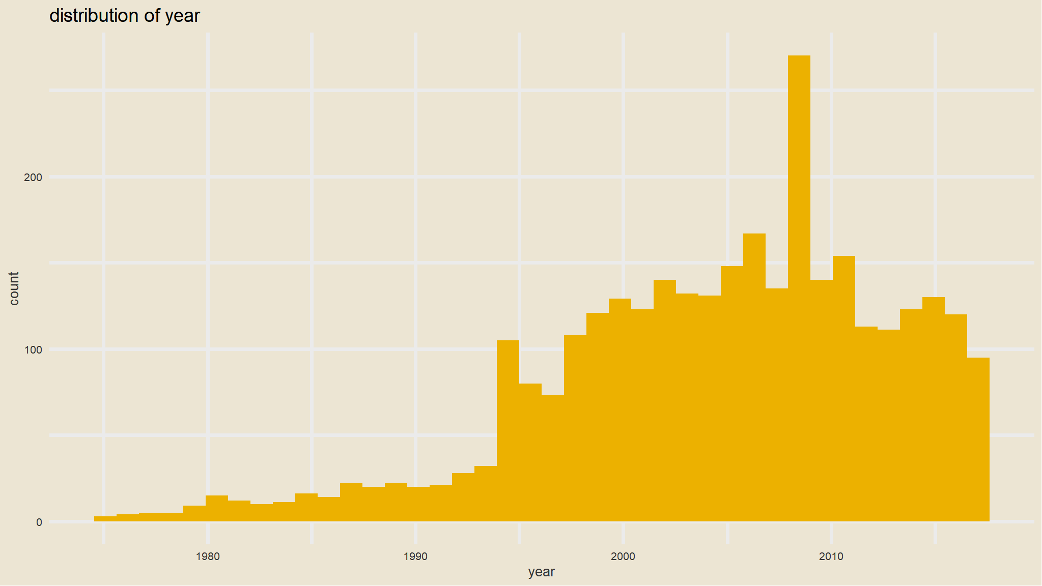
mov<-mov |> 
  filter(year>= 1975 & year < 2018)

ggplot(mov, aes(year)) + 
  geom_histogram(bins=40, fill=avatar_pal()(1))+
  theme_avatar()+
  labs(title="distribution of year")

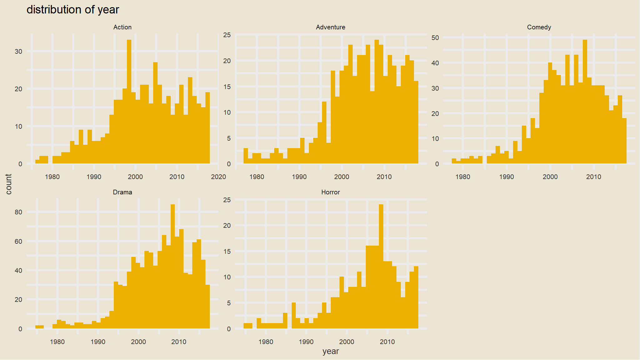
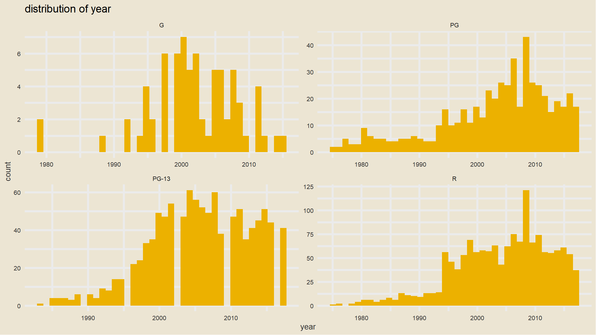
that looks awesome ,we can picture that by genre or rating as well

ggplot(mov, aes(year)) + 
  geom_histogram(bins=40, fill=avatar_pal()(1))+
  theme_avatar()+
  facet_wrap(~genre,scales="free")+
  labs(title="distribution of year")

ggplot(mov, aes(year)) + 
  geom_histogram(bins=40, fill=avatar_pal()(1))+
  theme_avatar()+
  facet_wrap(~mpaa_rating,scales="free")+
  labs(title="distribution of year")

Days the movies were released

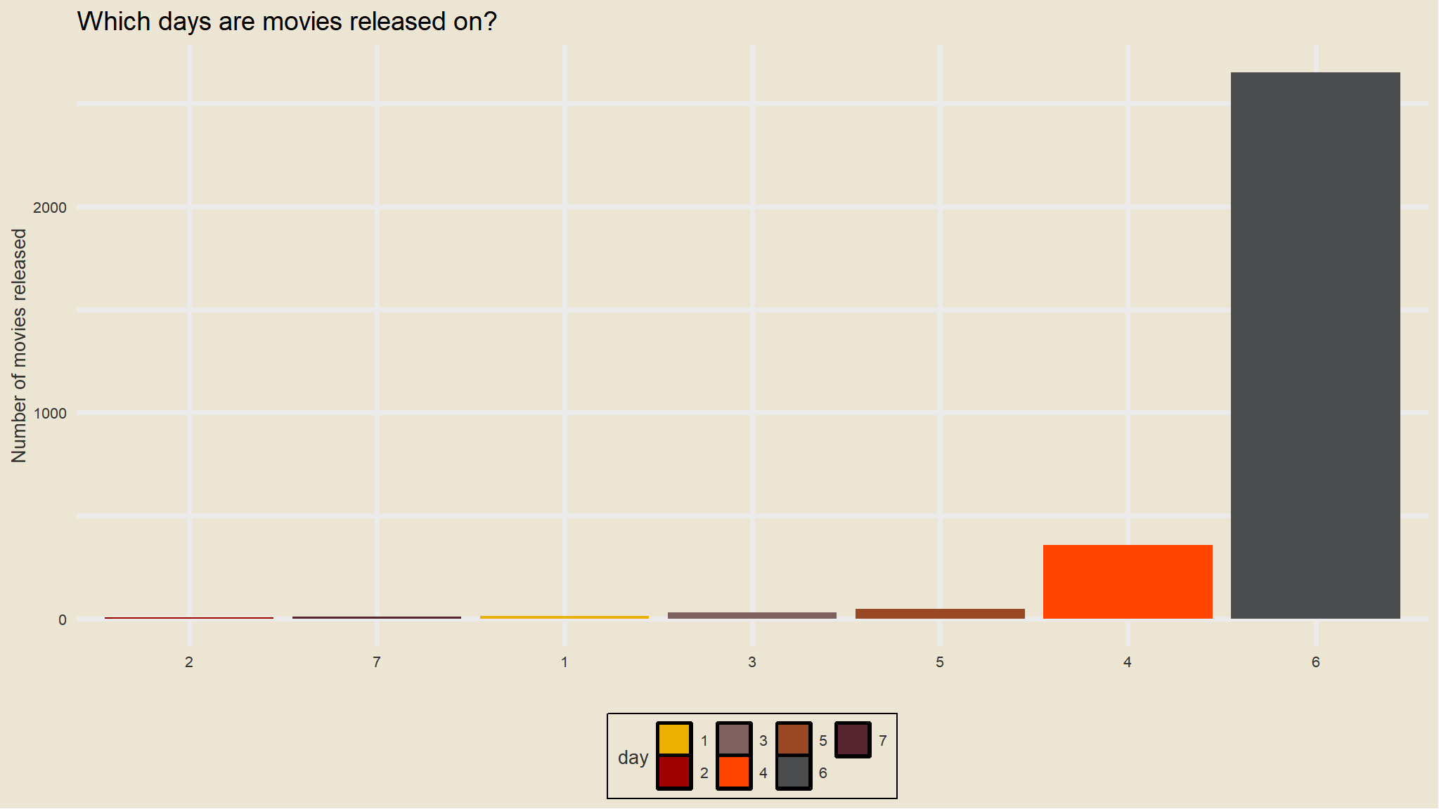
library(ggthemes)

mov |> 
  count(day, sort=TRUE) |> 
  ggplot(aes(y=n,x=fct_reorder(day,n),fill=day)) + 
  geom_col() + 
  labs(x="", y="Number of movies released", 
       title="Which days are movies released on?") + 
  theme_avatar() + scale_fill_avatar()

most movies were watched on a Friday (Friday night maybe)

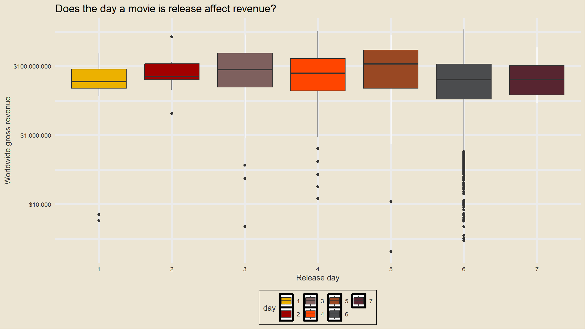
library(scales)
mov |> 
  ggplot(aes(day, worldwide_gross,fill=day)) + 
  geom_boxplot() + 
  scale_y_log10(labels=dollar_format()) +
  labs(x="Release day",
       y="Worldwide gross revenue", 
       title="Does the day a movie is release affect revenue?") + 
  scale_fill_avatar()+
  theme_avatar()

let us perfom a statistical test for this

Does the mean gross differ?

mov |> 
  group_by(day) |> 
  summarise(average=mean(worldwide_gross),
            median = median(worldwide_gross),
            std.dev= sd(worldwide_gross))
#> # A tibble: 7 × 4
#>   day      average     median    std.dev
#>   <fct>      <dbl>      <dbl>      <dbl>
#> 1 1      70256412.  36674010   78293203.
#> 2 2     141521289.  50446776. 233127207.
#> 3 3     177233110.  80013623  228434437.
#> 4 4     130794183.  62076141  178563855.
#> 5 5     194466996. 121318930. 216828529.
#> 6 6      90769834.  41166033  131301918.
#> 7 7      89889497.  41486381  114314385.

run an anova test on this!

model<-aov(worldwide_gross~day,data=mov)
summary(model)
#>               Df    Sum Sq   Mean Sq F value   Pr(>F)    
#> day            6 1.178e+18 1.963e+17   9.961 6.44e-11 ***
#> Residuals   3110 6.129e+19 1.971e+16                     
#> ---
#> Signif. codes:  0 '***' 0.001 '**' 0.01 '*' 0.05 '.' 0.1 ' ' 1

$H_0$ : there is no difference in means
$H_1$ : means are different

since p-value is less than 0.05 we reject null hypothesis and conclude that the difference in mean gross is statistically significant

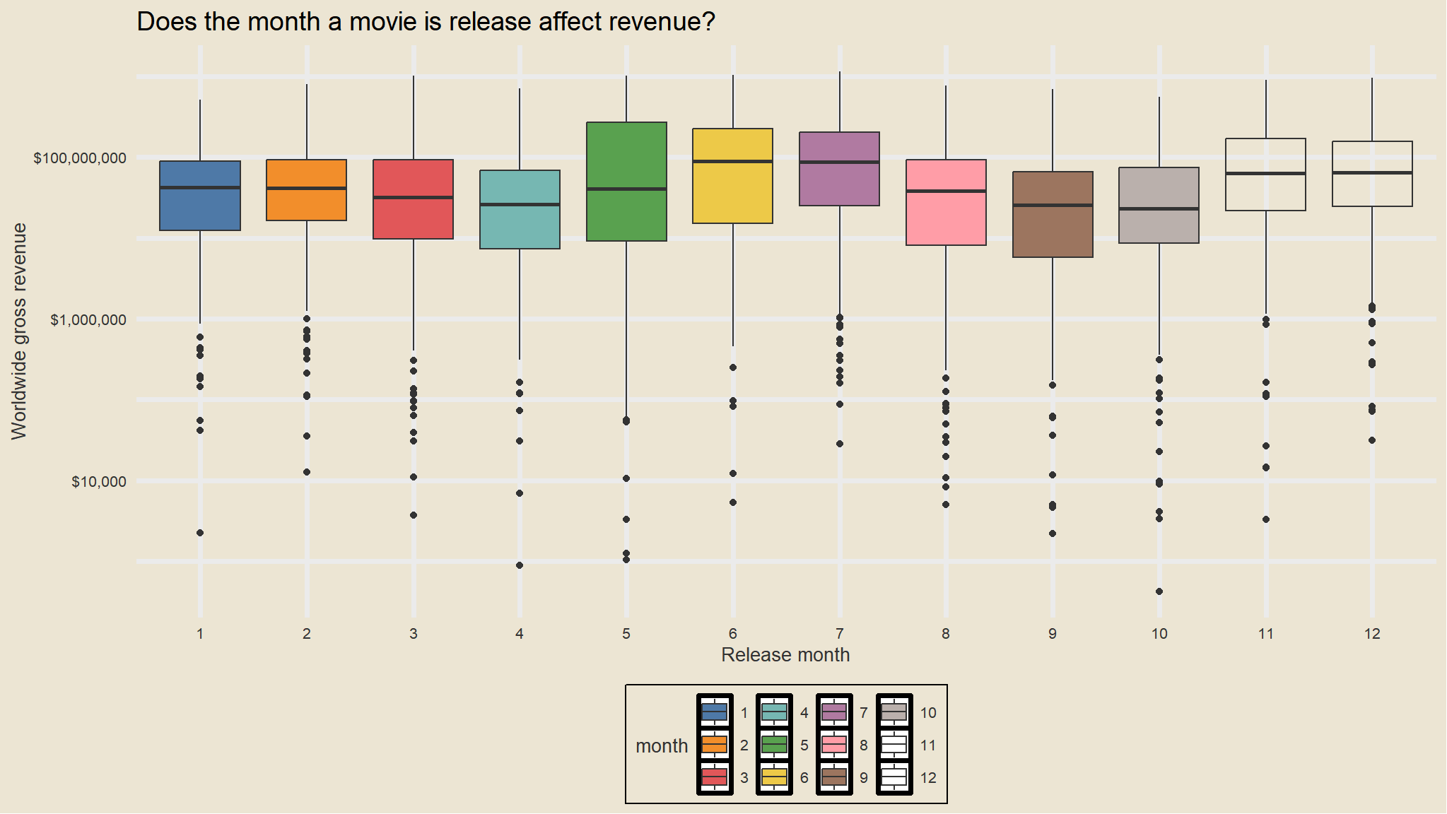
what about month?

library(scales)
mov |> 
  ggplot(aes(factor(month), worldwide_gross,fill=factor(month))) + 
  geom_boxplot() + 
  scale_y_log10(labels=dollar_format()) +
  labs(x="Release month",
       y="Worldwide gross revenue", 
       title="Does the month a movie is release affect revenue?",
       fill="month") + 
  scale_fill_tableau()+
  theme_avatar()

mov |> 
  group_by(month) |> 
  summarize(rev=mean(worldwide_gross))

mov |> 
  mutate(month=factor(month, ordered=FALSE)) %$%
  lm(worldwide_gross~month) |> 
  summary()

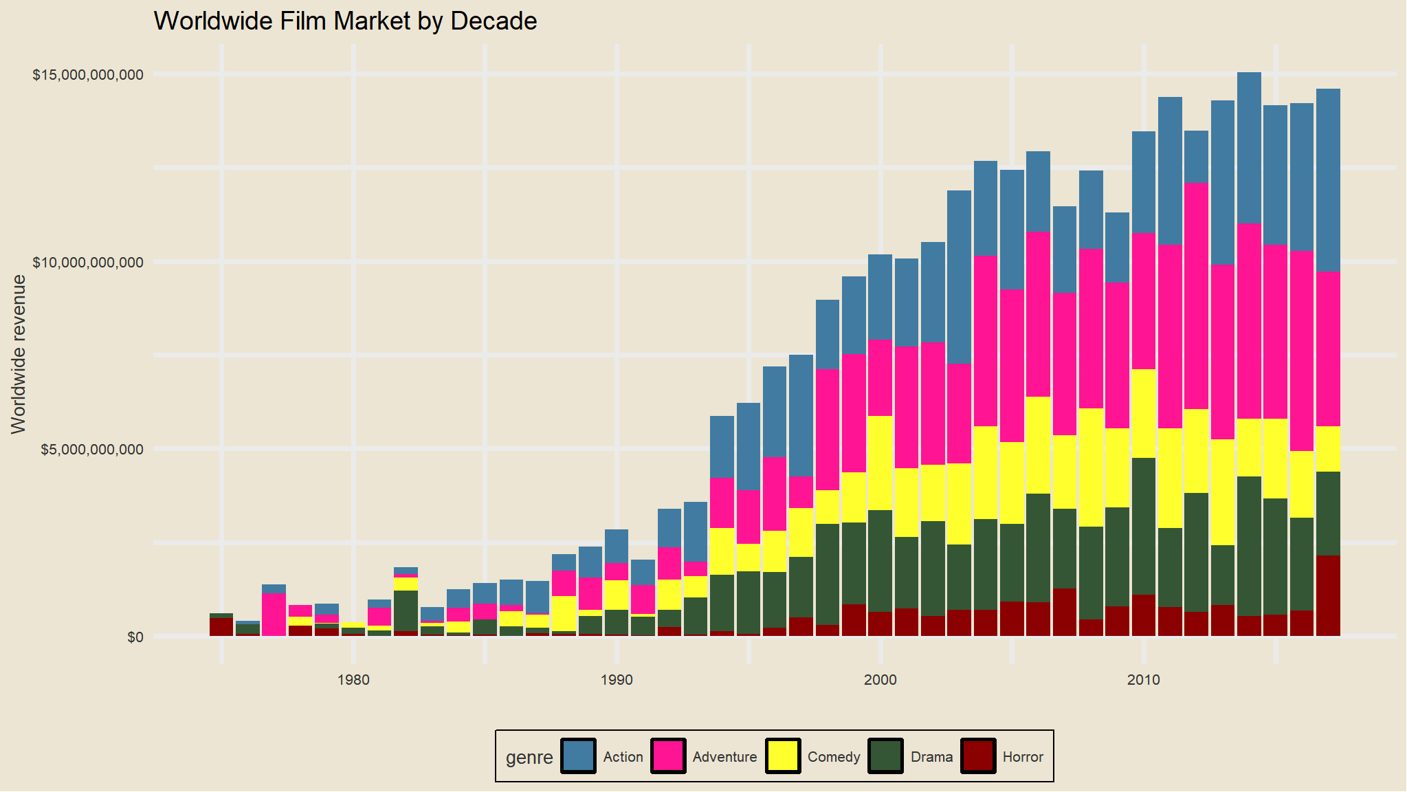
What does the worldwide movie market look like by decade? Let’s first group by year and genre and compute the sum of the worldwide gross revenue. After we do that, let’s plot a barplot showing year on the x-axis and the sum of the revenue on the y-axis, where we’re passing the genre variable to the fill aesthetic of the bar.

mov |> 
  group_by(year, genre) |> 
  summarise(revenue=sum(worldwide_gross)) |> 
  ggplot(aes(year, revenue)) + 
  geom_col(aes(fill=genre)) + 
  scale_y_continuous(labels=dollar_format()) + 
  labs(x="", y="Worldwide revenue", title="Worldwide Film Market by Decade")+
  theme_avatar()+
  scale_fill_gravityFalls()

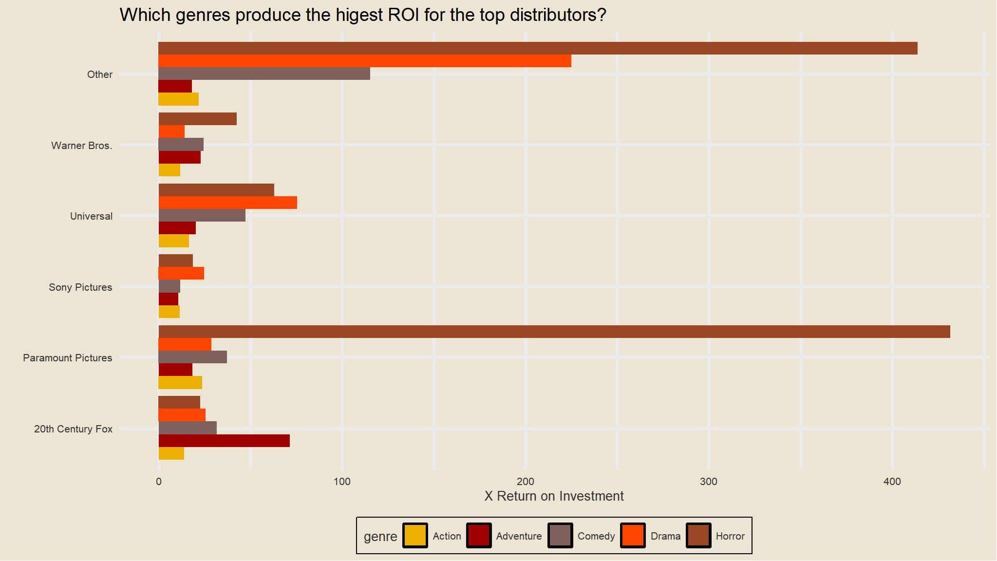
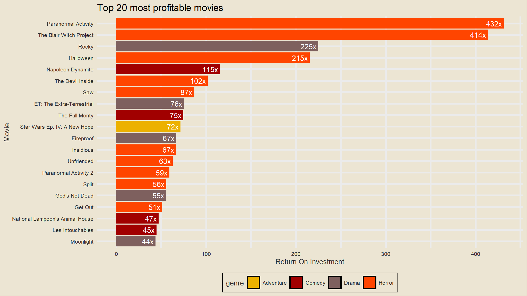
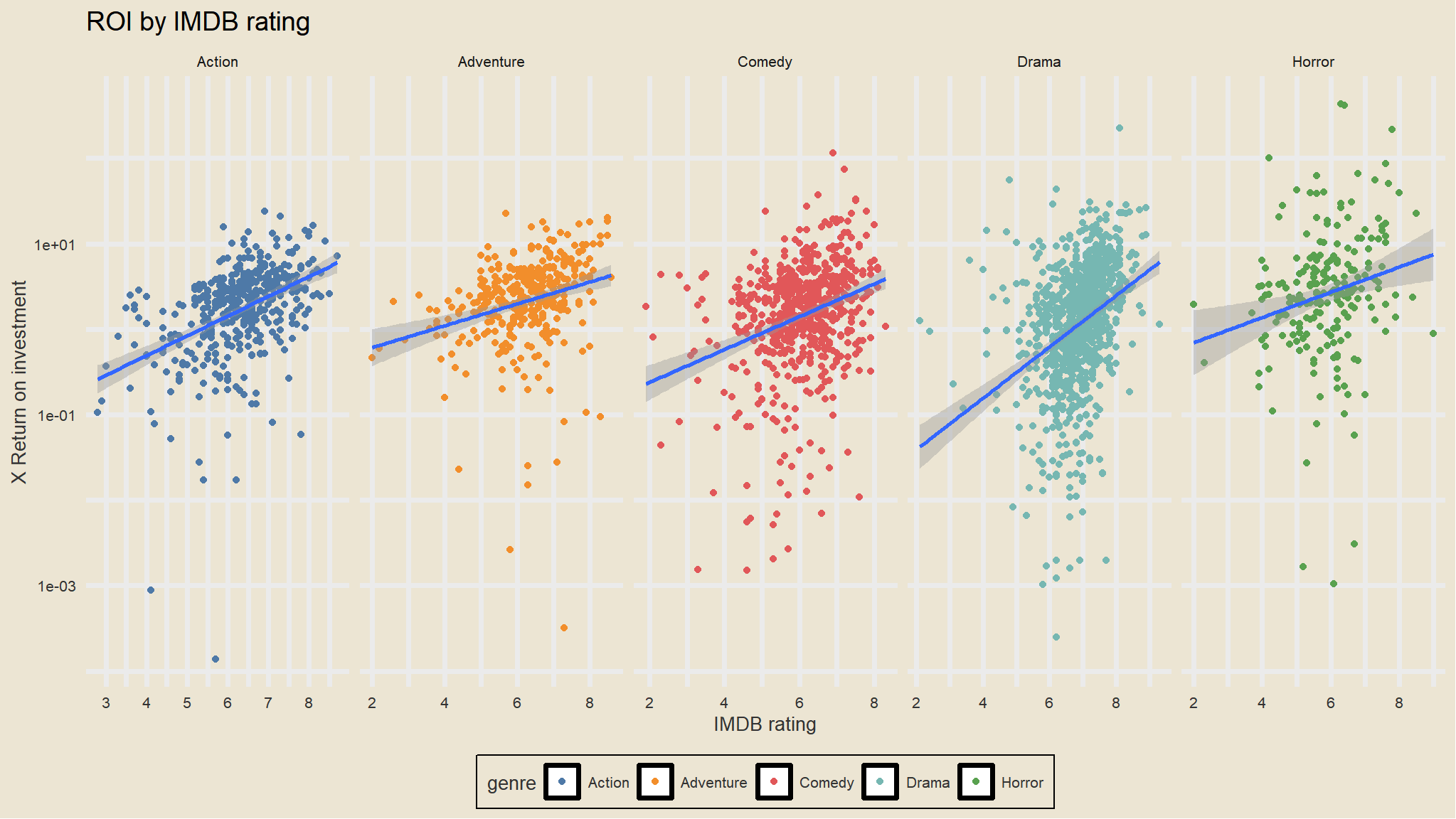
Which genres produce the highest Return on investment?

looks like horror movies and drama take the lead .

next up

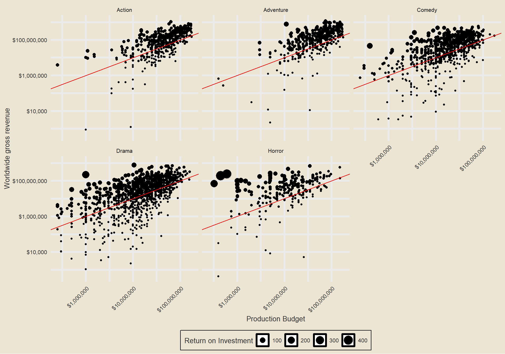
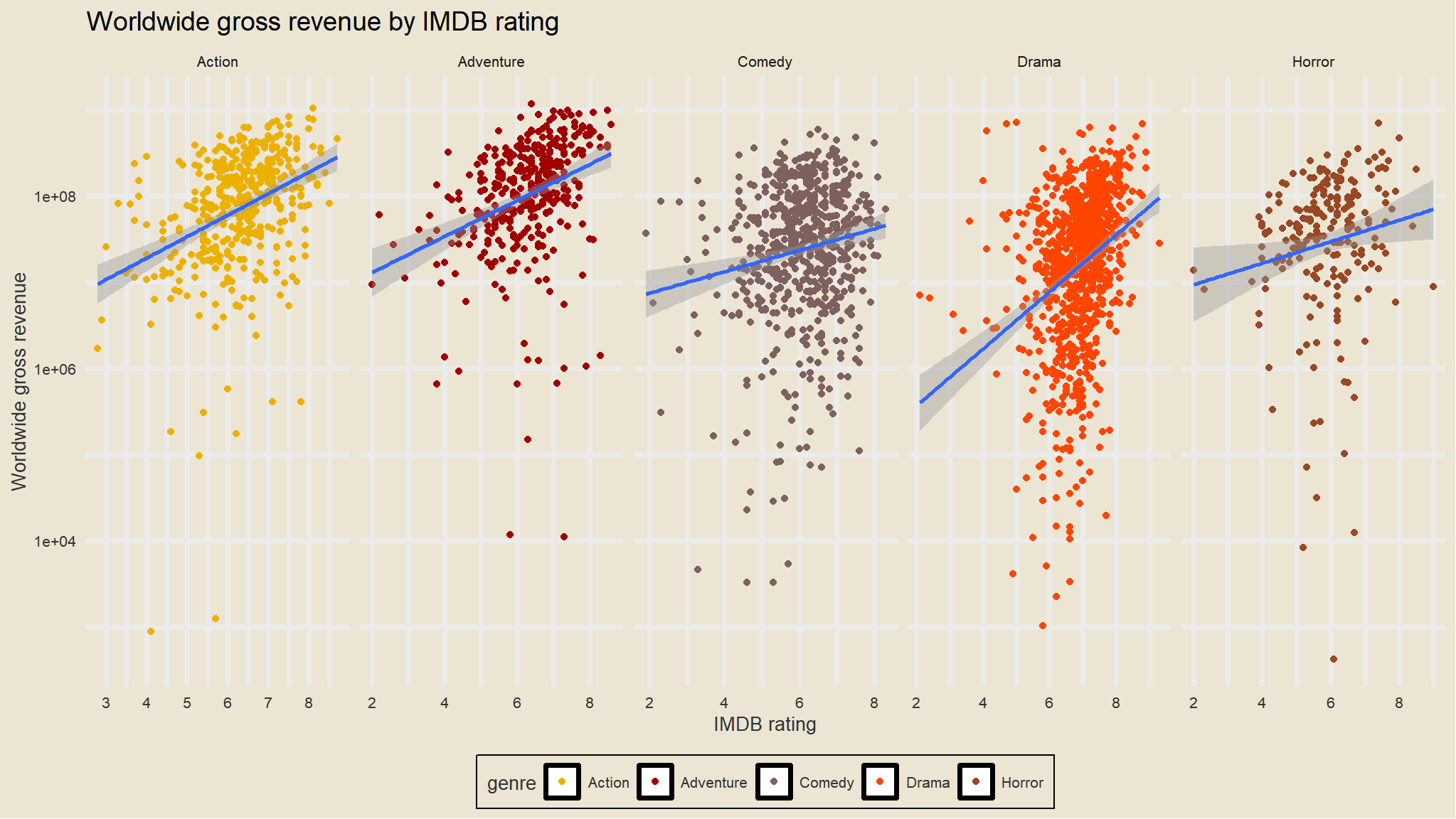
Let’s make a scatter plot showing the worldwide gross revenue over the production budget and let us facet by genre.

mov |>
  ggplot(aes(production_budget, worldwide_gross)) +
  geom_point(aes(size = roi)) +
  geom_abline(slope = 1, intercept = 0, col = "red") +
  facet_wrap( ~ genre) +
  theme_avatar()+
  scale_x_log10(labels = dollar_format()) +
  scale_y_log10(labels = dollar_format()) +
  theme(axis.text.x = element_text(angle = 45, hjust = 1)) +
  labs(x = "Production Budget", 
       y = "Worldwide gross revenue", 
       size = "Return on Investment")

Generally most of the points lie above the “breakeven” line. This is good – if movies weren’t profitable they wouldn’t keep making them. Proportionally there seem to be many more larger points in the Horror genre, indicative of higher ROI.

which are some of the most profitable movies

mov |> 
  arrange(desc(roi)) |> 
  head(20) |> 
  mutate(movie=fct_reorder(movie, roi)) |>
  ggplot(aes(movie, roi)) +
  geom_col(aes(fill=genre)) + 
  scale_fill_avatar()+
  theme_avatar()+
  labs(x="Movie", 
       y="Return On Investment", 
       title="Top 20 most profitable movies") + 
  coord_flip() + 
  geom_text(aes(label=paste0(round(roi), "x "), hjust=1), col="white")

let’s look at movie ratings

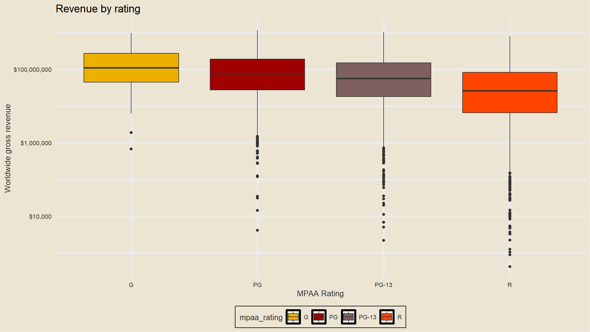
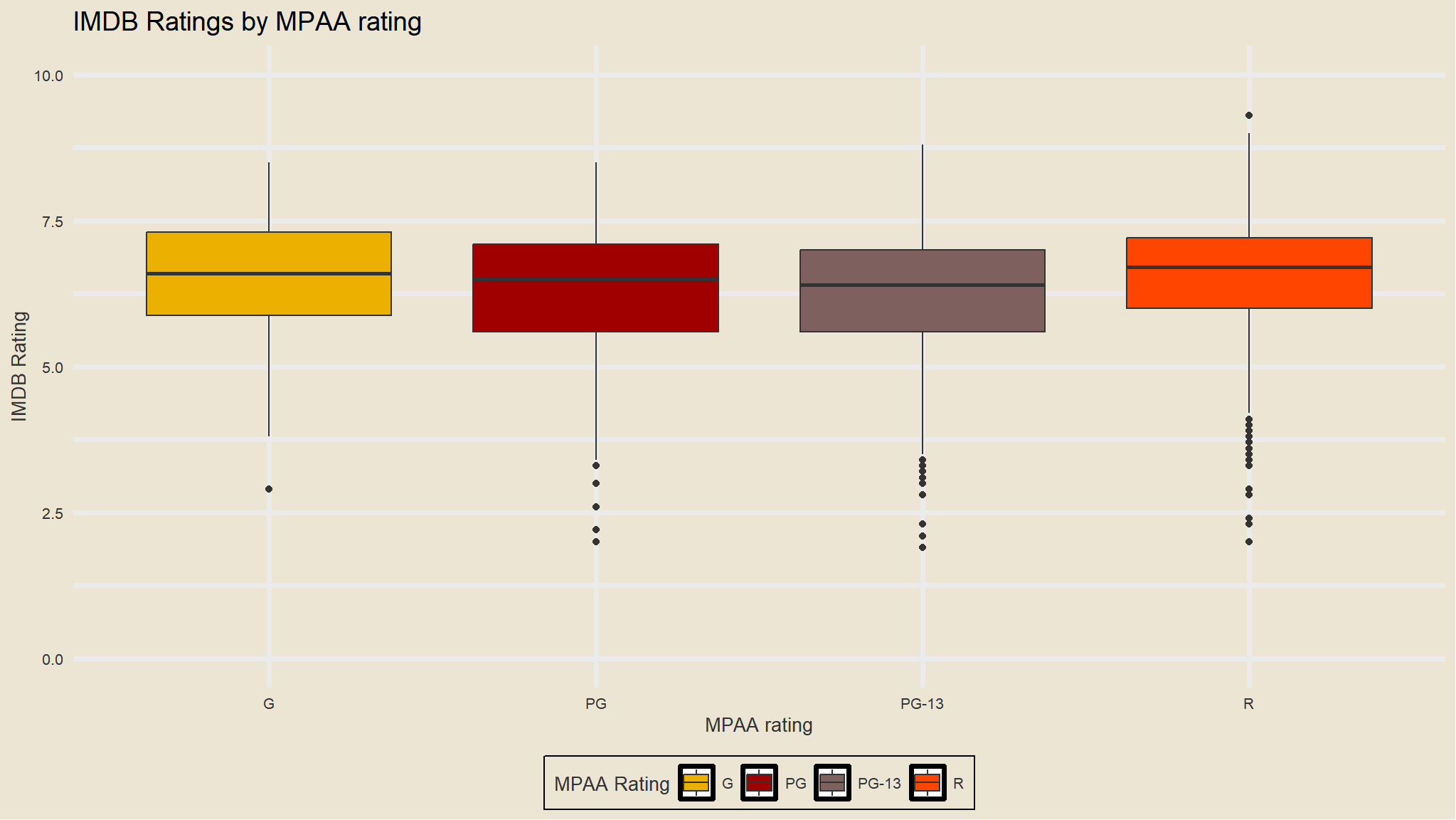
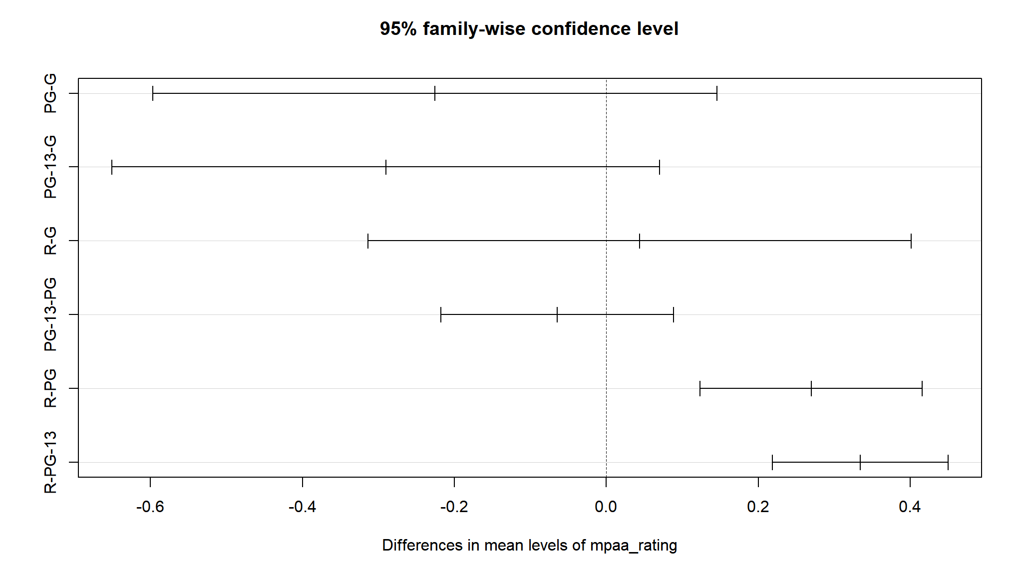
R-rated movies have a lower average revenue but ROI isn’t substantially less. We can see that while G-rated movies have the highest mean revenue, there were relatively few of them produced, and had a lower total revenue. There were more R-rated movies, but PG-13 movies really drove the total revenue worldwide.

mov |>
  group_by(mpaa_rating) |>
  summarize(
    meanrev = mean(worldwide_gross),
    totrev = sum(worldwide_gross),
    roi = mean(roi),
    number = n()
  )
#> # A tibble: 4 × 5
#>   mpaa_rating    meanrev       totrev   roi number
#>   <fct>            <dbl>        <dbl> <dbl>  <int>
#> 1 G           189913348   13863674404  4.42     73
#> 2 PG          147227422.  78324988428  4.64    532
#> 3 PG-13       113477939. 120173136920  3.06   1059
#> 4 R            63627931.  92451383780  4.42   1453

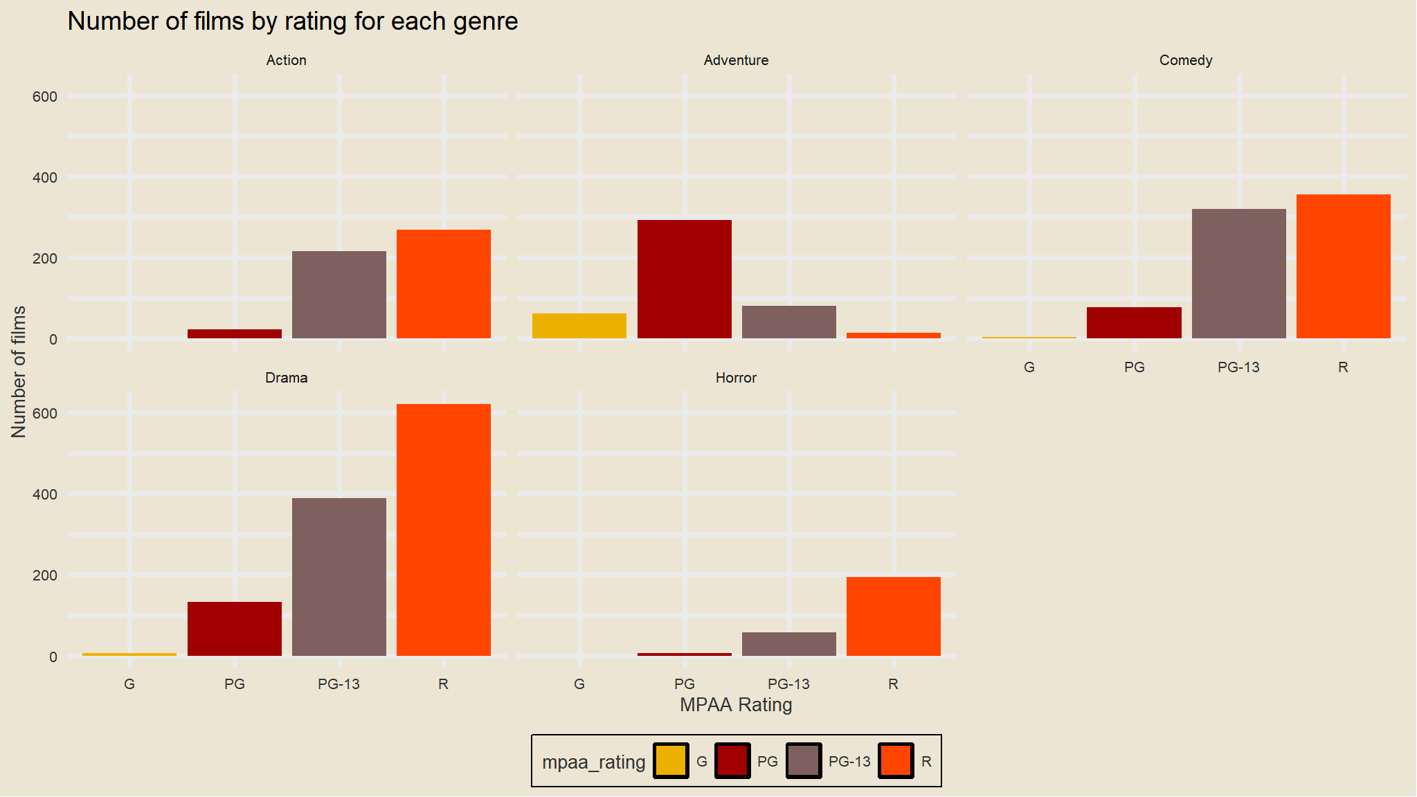
Are there fewer R-rated movies being produced? Not really. Let’s look at the overall number of movies with any particular rating faceted by genre.

mov |> 
  count(mpaa_rating, genre) |> 
  ggplot(aes(mpaa_rating, n,fill=mpaa_rating)) + 
  geom_col() + 
  theme_avatar()+
  scale_fill_avatar()+
  facet_wrap(~genre) +
  labs(x="MPAA Rating",
       y="Number of films", 
       title="Number of films by rating for each genre")

What about the distributions of ratings?

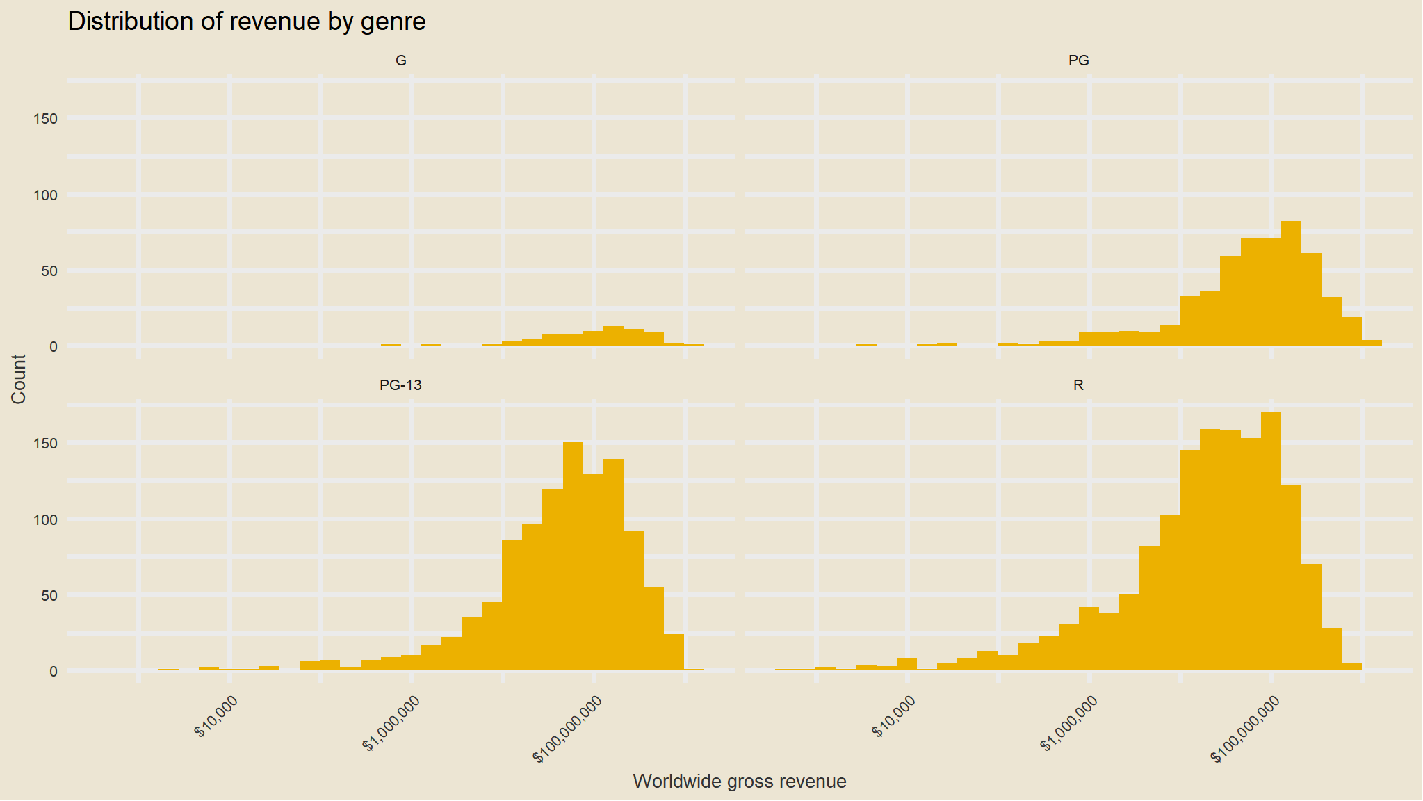
mov |> 
  ggplot(aes(worldwide_gross)) + 
  geom_histogram(fill=avatar_pal()(1)) + 
  facet_wrap(~mpaa_rating) +
  theme_avatar()+
  scale_x_log10(labels=dollar_format()) + 
  labs(x="Worldwide gross revenue", 
       y="Count",
       title="Distribution of revenue by genre")+
  theme(axis.text.x = element_text(angle = 45, hjust = 1))

mov |> 
  ggplot(aes(mpaa_rating, worldwide_gross,fill=mpaa_rating)) + 
  scale_fill_avatar()+
  geom_boxplot() + 
  theme_avatar()+
  scale_y_log10(labels=dollar_format()) + 
  labs(x="MPAA Rating", y="Worldwide gross revenue", title="Revenue by rating")

Yes, on average G-rated movies look to perform better. But there aren’t that many of them being produced, and they aren’t bringing in the lions share of revenue.

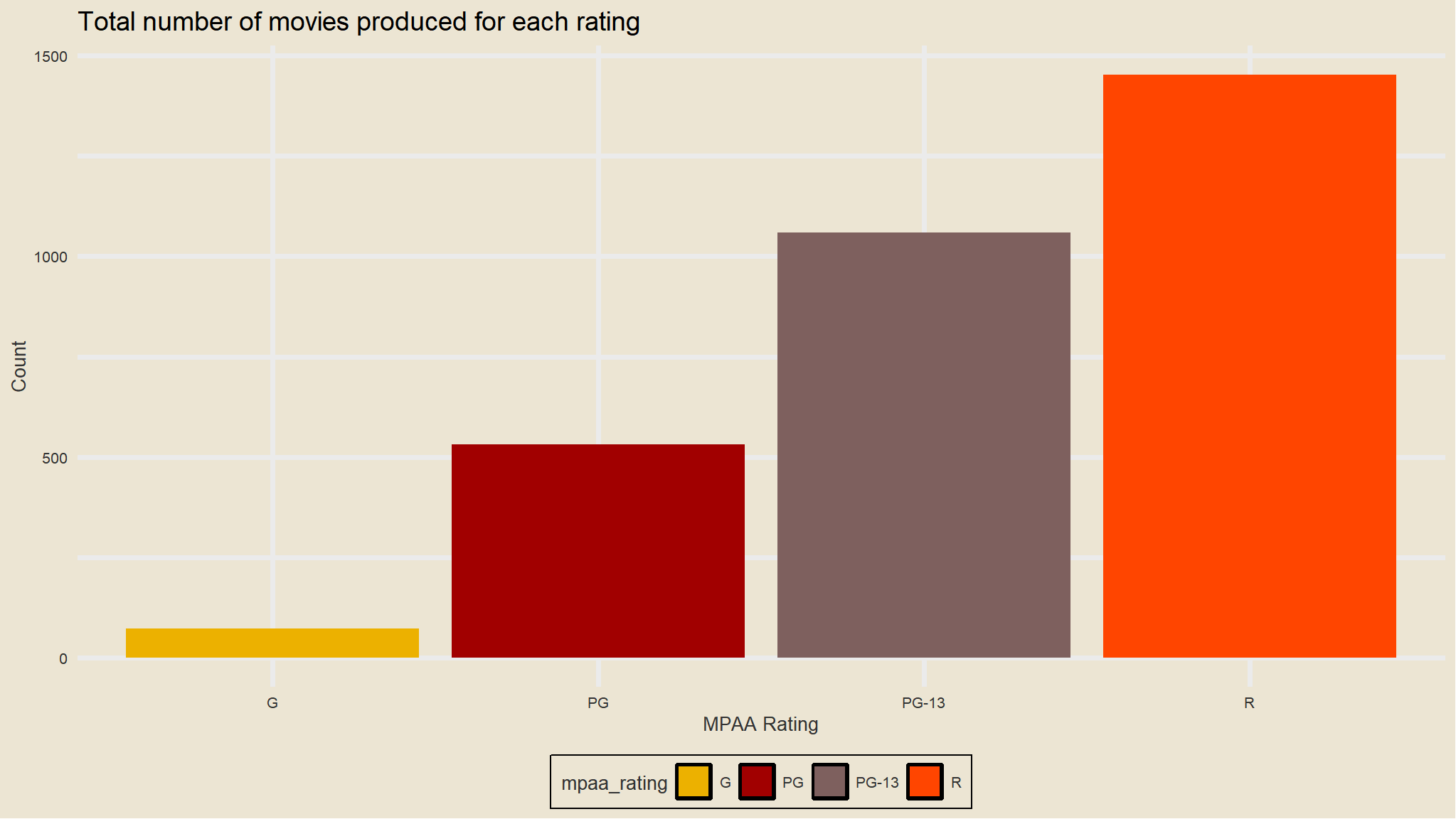
mov |> 
  count(mpaa_rating) |> 
  ggplot(aes(mpaa_rating, n,fill=mpaa_rating)) + 
  theme_avatar()+
  scale_fill_avatar()+
  geom_col() + 
  labs(x="MPAA Rating", 
       y="Count",
       title="Total number of movies produced for each rating")

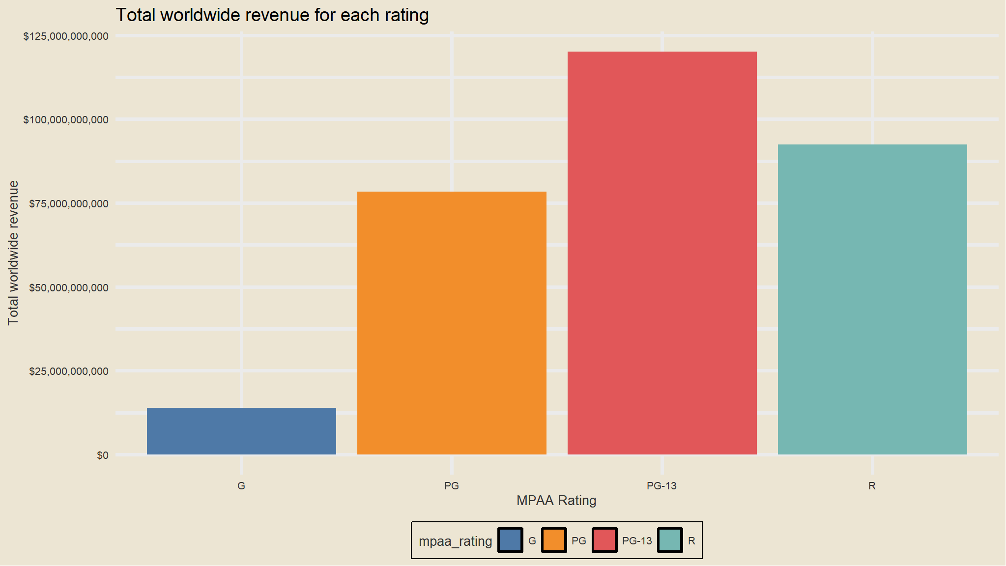
mov |> 
  group_by(mpaa_rating) |> 
  summarize(total_revenue=sum(worldwide_gross)) |> 
  ggplot(aes(mpaa_rating, total_revenue ,fill=mpaa_rating)) + 
  geom_col() + 
  scale_fill_tableau()+
  theme_avatar()+
  scale_y_continuous(label=dollar_format()) + 
  labs(x="MPAA Rating", 
       y="Total worldwide revenue",
       title="Total worldwide revenue for each rating")

PG-13 Seems to bring in more revenue worldwide

but wait , is there any association between genre and mpaa_rating?

# Create frequency table, save for reuse
ptable <- mov %>%           # Save table for reuse
  select(mpaa_rating, genre) %>%  # Variables for table
  table() %>%              # Create 2 x 2 table
  print()                  # Show table
#>            genre
#> mpaa_rating Action Adventure Comedy Drama Horror
#>       G          0        62      4     7      0
#>       PG        23       293     77   133      6
#>       PG-13    215        80    319   388     57
#>       R        268        14    356   621    194

CHI-SQUARED TEST

# Get chi-squared test for mpaa_rating and genre
ptable %>% chisq.test()
#> 
#>  Pearson's Chi-squared test
#> 
#> data:  .
#> X-squared = 1343.7, df = 12, p-value < 2.2e-16

great ,p-value is less than 0.05 hence we can tell that genre and mpaa_rating are greatly associated .

let us Join to IMDB reviews dataset and get more insights

imdb <- read_csv("movies_imdb.csv")
head(imdb)

let us inner join the two datasets together

do not worry , i will share another tutorial on performing joins exclusively ,otherwise you can check one of my tutorials that compares SQL and R

movimdb <- inner_join(mov, imdb, by="movie")
head(movimdb)

What`s next?

let’s see some correlations here

Correlation

Correlation measures the strength and direction of association between two variables. There are three common correlation tests: the Pearson product moment (Pearson’s r), Spearman’s rank-order (Spearman’s rho), and Kendall’s tau (Kendall’s tau).

Use the Pearson’s r if both variables are quantitative (interval or ratio), normally distributed, and the relationship is linear with homoscedastic residuals.

The Spearman’s rho and Kendal’s tao correlations are non-parametric measures, so they are valid for both quantitative and ordinal variables and do not carry the normality and homoscedasticity conditions. However, non-parametric tests have less statistical power than parametric tests, so only use these correlations if Pearson does not apply.

let’s correlate

df<- mov |> 
  select_if(is.numeric)

# Correlation matrix for data frame
df %>% cor()
#>                   production_budget domestic_gross worldwide_gross         roi
#> production_budget        1.00000000     0.56946432      0.64987504 -0.08666254
#> domestic_gross           0.56946432     1.00000000      0.92468680  0.18692435
#> worldwide_gross          0.64987504     0.92468680      1.00000000  0.16047814
#> roi                     -0.08666254     0.18692435      0.16047814  1.00000000
#> pct_domestic            -0.31400653    -0.17286869     -0.34792146 -0.05975148
#> year                     0.10558412    -0.06889791      0.03379454 -0.07545929
#> month                    0.02019088     0.03681648      0.02885615  0.02167627
#>                   pct_domestic        year       month
#> production_budget  -0.31400653  0.10558412  0.02019088
#> domestic_gross     -0.17286869 -0.06889791  0.03681648
#> worldwide_gross    -0.34792146  0.03379454  0.02885615
#> roi                -0.05975148 -0.07545929  0.02167627
#> pct_domestic        1.00000000 -0.32547167 -0.05291129
#> year               -0.32547167  1.00000000 -0.07293380
#> month              -0.05291129 -0.07293380  1.00000000

yooogh ,that looks a bit messy!

# Fewer decimal places
df %>%
  cor() %>%     # Compute correlations
  round(2) %>%  # Round to 2 decimals
  print()
#>                   production_budget domestic_gross worldwide_gross   roi
#> production_budget              1.00           0.57            0.65 -0.09
#> domestic_gross                 0.57           1.00            0.92  0.19
#> worldwide_gross                0.65           0.92            1.00  0.16
#> roi                           -0.09           0.19            0.16  1.00
#> pct_domestic                  -0.31          -0.17           -0.35 -0.06
#> year                           0.11          -0.07            0.03 -0.08
#> month                          0.02           0.04            0.03  0.02
#>                   pct_domestic  year month
#> production_budget        -0.31  0.11  0.02
#> domestic_gross           -0.17 -0.07  0.04
#> worldwide_gross          -0.35  0.03  0.03
#> roi                      -0.06 -0.08  0.02
#> pct_domestic              1.00 -0.33 -0.05
#> year                     -0.33  1.00 -0.07
#> month                    -0.05 -0.07  1.00

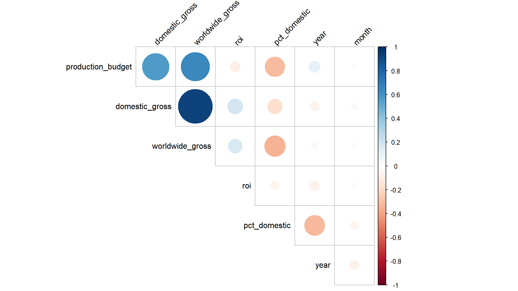
Visualize correlation matrix with corrplot() from corrplot package

library(corrplot)

df %>%
  cor() %>%
  corrplot(
    type   = "upper",     # Matrix: full, upper, or lower
    diag   = F,           # Remove diagonal
    order  = "original",  # Order for labels
    tl.col = "black",     # Font color
    tl.srt = 45           # Label angle
  )

production cost ,world wide gross and domestic gross all seem to be inter-correlated
but is it significant?

# SINGLE CORRELATION #######################################

# Use cor.test() to test one pair of variables at a time.
# cor.test() gives r, the hypothesis test, and the
# confidence interval. This command uses the "exposition
# pipe," %$%, from magrittr, which passes the columns from
# the data frame (and not the data frame itself)

df %$% cor.test(production_budget,worldwide_gross)
#> 
#>  Pearson's product-moment correlation
#> 
#> data:  production_budget and worldwide_gross
#> t = 47.722, df = 3115, p-value < 2.2e-16
#> alternative hypothesis: true correlation is not equal to 0
#> 95 percent confidence interval:
#>  0.6291207 0.6697034
#> sample estimates:
#>      cor 
#> 0.649875

off course yes ,the correlation is statistically significant
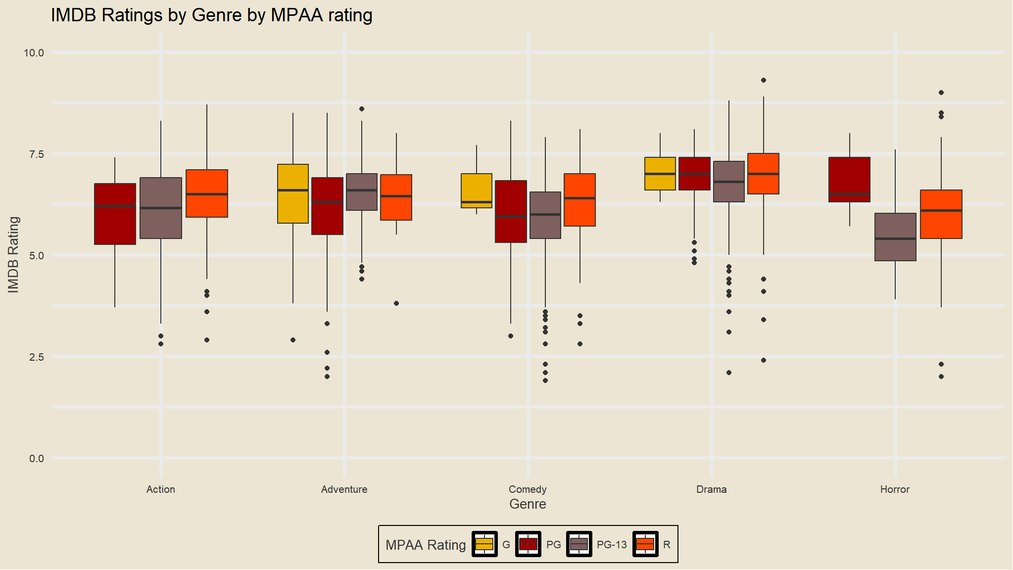
Separately for each MPAA rating, i will display the mean IMDB rating and mean number of votes cast.

#> # A tibble: 4 × 3
#>   mpaa_rating meanimdb meanvotes
#>   <fct>          <dbl>     <dbl>
#> 1 G               6.54   132015.
#> 2 PG              6.31    81841.
#> 3 PG-13           6.25   102740.
#> 4 R               6.58   107575.

let’s try to visualise the above results using boxplots and compare means

as seen from the means ,there seem to quite similar mean ratings here ,let’s run an ANOVA

model<-aov(imdb~mpaa_rating,data=movimdb)
summary(model)
#>               Df Sum Sq Mean Sq F value   Pr(>F)    
#> mpaa_rating    3   63.9  21.314   20.57 3.57e-13 ***
#> Residuals   2587 2680.0   1.036                     
#> ---
#> Signif. codes:  0 '***' 0.001 '**' 0.01 '*' 0.05 '.' 0.1 ' ' 1

comments

p-value is less than 0.05 hence there seem to be significant mean differences here

but which ratings actually differ?

lets run a post-hoc analysis

model_tukey<-TukeyHSD(model)
model_tukey
#>   Tukey multiple comparisons of means
#>     95% family-wise confidence level
#> 
#> Fit: aov(formula = imdb ~ mpaa_rating, data = movimdb)
#> 
#> $mpaa_rating
#>                 diff        lwr        upr     p adj
#> PG-G     -0.22557339 -0.5969917 0.14584492 0.4011330
#> PG-13-G  -0.29020880 -0.6507315 0.07031389 0.1634754
#> R-G       0.04403339 -0.3135888 0.40165555 0.9890254
#> PG-13-PG -0.06463541 -0.2176996 0.08842880 0.6984264
#> R-PG      0.26960678  0.1235053 0.41570829 0.0000131
#> R-PG-13   0.33424219  0.2186105 0.44987391 0.0000000

the output suggests that the pairs R and PG And R and P-13 seem to have statistically significant mean differences
we can also visualise these results below

plot(model_tukey)

let’s do it for the genre as well

we can repeat the same analysis using the genre variable now

#> # A tibble: 5 × 3
#>   genre     meanimdb meanvotes
#>   <fct>        <dbl>     <dbl>
#> 1 Action        6.28   154681.
#> 2 Adventure     6.27   130027.
#> 3 Comedy        6.08    71288.
#> 4 Drama         6.88    91101.
#> 5 Horror        5.90    89890.

model<-aov(imdb~genre,data=movimdb)
summary(model)
#>               Df Sum Sq Mean Sq F value Pr(>F)    
#> genre          4  352.3   88.07   95.22 <2e-16 ***
#> Residuals   2586 2391.6    0.92                   
#> ---
#> Signif. codes:  0 '***' 0.001 '**' 0.01 '*' 0.05 '.' 0.1 ' ' 1