Data Transformation and Explanatory analysis

Data wrangling

data wrangling

munging

statistics

Author

Bongani Ncube

Published

27 January 2024

Objectives

Welcome to yet another R blog on data analysis and wranling using R At the end of this tutorial you will:

understand the role of data wrangling
understand the basic capabilities of dplyr
acquire skills to perform common data wrangling using dplyr,stringr,tidyr and forcats packages

What is data wrangling?

Note

Data wrangling is also known as Data Munging or Data Transformation. It is loosely the process of manually converting or mapping data from one “raw” form into another format. The process allows for more convenient consumption of the data. Data analysts typically spend the majority of their time in the process of data wrangling compared to the actual analysis of the data.

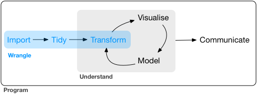
Common data wrangling processes

The common data wrangling processes include:

Note

reducing the size of dataset by selecting certain variables (or columns)
generating new variable from existing variables
sorting observation of a variable
grouping observations based on certain criteria
reducing variables to groups in order to estimate summary statistic

Use tidyverse functions for achieving this!

already have a blog about these functions

Note

dplyr::select() - to select a number of variables from a dataframe
dplyr::mutate() - to generate a new variable from existing variables
dplyr::arrange()- to sort observation of a variable
dplyr::filter() - to group observations that fulfil certain criteria
dplyr::group_by() and dplyr::summarize() - to reduce variable to groups in order to provide summary statistic

setup

library(tidyverse)
library(lubridate)

new_data <- read_csv("recipe_site_traffic_2212.csv")
dim(new_data)
#> [1] 947   8
names(new_data)
#> [1] "recipe"       "calories"     "carbohydrate" "sugar"        "protein"     
#> [6] "category"     "servings"     "high_traffic"

Take a peek at the recipe site dataset.

Note

The dataset contains:

947 observations
8 variables

glimpse(new_data)
#> Rows: 947
#> Columns: 8
#> $ recipe       <chr> "001", "002", "003", "004", "005", "006", "007", "008", "…
#> $ calories     <dbl> NA, 35.48, 914.28, 97.03, 27.05, 691.15, 183.94, 299.14, …
#> $ carbohydrate <dbl> NA, 38.56, 42.68, 30.56, 1.85, 3.46, 47.95, 3.17, 3.78, 4…
#> $ sugar        <dbl> NA, 0.66, 3.09, 38.63, 0.80, 1.65, 9.75, 0.40, 3.37, 3.99…
#> $ protein      <dbl> NA, 0.92, 2.88, 0.02, 0.53, 53.93, 46.71, 32.40, 3.79, 11…
#> $ category     <chr> "Pork", "Potato", "Breakfast", "Beverages", "Beverages", …
#> $ servings     <chr> "6", "4", "1", "4", "4", "2", "4", "4", "6", "2", "1", "6…
#> $ high_traffic <chr> "High", "High", NA, "High", NA, "High", NA, NA, "High", N…

Next, we examine the first five observations of the data. The rest of the observations are not shown. You can also see the types of variables:

chr (character),
int (integer),
dbl (double)

new_data|> head(n = 5)
#> # A tibble: 5 × 8
#>   recipe calories carbohydrate sugar protein category  servings high_traffic
#>   <chr>     <dbl>        <dbl> <dbl>   <dbl> <chr>     <chr>    <chr>       
#> 1 001        NA          NA    NA      NA    Pork      6        High        
#> 2 002        35.5        38.6   0.66    0.92 Potato    4        High        
#> 3 003       914.         42.7   3.09    2.88 Breakfast 1        <NA>        
#> 4 004        97.0        30.6  38.6     0.02 Beverages 4        High        
#> 5 005        27.0         1.85  0.8     0.53 Beverages 4        <NA>

Select variables, generate new variable and rename variable

We will work with these functions.

dplyr::select()
dplyr::mutate() and
dplyr::rename()

Select variables using `dplyr::select()`

When you work with large datasets with many columns, it is sometimes easier to select only the necessary columns to reduce the dataset size. This is possible by creating a smaller dataset (fewer variables). Then you can work on the initial part of data analysis with this smaller dataset. This will greatly help data exploration.

Note

however for this exercise we gonna need all the variables for exploration so we will select everything

(new_data <- new_data|> 
  dplyr::select(everything()))
#> # A tibble: 947 × 8
#>    recipe calories carbohydrate sugar protein category     servings high_traffic
#>    <chr>     <dbl>        <dbl> <dbl>   <dbl> <chr>        <chr>    <chr>       
#>  1 001        NA          NA    NA      NA    Pork         6        High        
#>  2 002        35.5        38.6   0.66    0.92 Potato       4        High        
#>  3 003       914.         42.7   3.09    2.88 Breakfast    1        <NA>        
#>  4 004        97.0        30.6  38.6     0.02 Beverages    4        High        
#>  5 005        27.0         1.85  0.8     0.53 Beverages    4        <NA>        
#>  6 006       691.          3.46  1.65   53.9  One Dish Me… 2        High        
#>  7 007       184.         48.0   9.75   46.7  Chicken Bre… 4        <NA>        
#>  8 008       299.          3.17  0.4    32.4  Lunch/Snacks 4        <NA>        
#>  9 009       539.          3.78  3.37    3.79 Pork         6        High        
#> 10 010       248.         48.5   3.99  114.   Chicken      2        <NA>        
#> # ℹ 937 more rows

extending `select` verb

Note

sometimes it is necessary to perform conditional selection on variables because + at times you need only numerical variables for correlations + you may only need categorical variables for testing independence

for such a case we can use functions such as select_if

new_data |> select_if(is.numeric)
#> # A tibble: 947 × 4
#>    calories carbohydrate sugar protein
#>       <dbl>        <dbl> <dbl>   <dbl>
#>  1     NA          NA    NA      NA   
#>  2     35.5        38.6   0.66    0.92
#>  3    914.         42.7   3.09    2.88
#>  4     97.0        30.6  38.6     0.02
#>  5     27.0         1.85  0.8     0.53
#>  6    691.          3.46  1.65   53.9 
#>  7    184.         48.0   9.75   46.7 
#>  8    299.          3.17  0.4    32.4 
#>  9    539.          3.78  3.37    3.79
#> 10    248.         48.5   3.99  114.  
#> # ℹ 937 more rows

the code above will only select variables of class numeric

Generate new variable using `mutate()`

With mutate(), you can generate a new variable. For example, in the dataset new_data, we want to create a new variable named log_calories which is a log transformation of calories .

\[log\_calories=\log(calories)\]

And let’s observe the first five observations:

new_data <- new_data|> 
  dplyr::mutate(log_calories = log(calories))

new_data |> 
  dplyr::select(log_calories,calories,sugar,category)|> 
  slice_head(n = 5)
#> # A tibble: 5 × 4
#>   log_calories calories sugar category 
#>          <dbl>    <dbl> <dbl> <chr>    
#> 1        NA        NA   NA    Pork     
#> 2         3.57     35.5  0.66 Potato   
#> 3         6.82    914.   3.09 Breakfast
#> 4         4.58     97.0 38.6  Beverages
#> 5         3.30     27.0  0.8  Beverages

extending `mutate` function

it is often wise to perform conditional mutations on data

Note

sometimes it is necessary to perform conditional mutation on variables such that + you only mutate is a certain condition is met

we often use mutate_if() ,mutate_at and mutate_all to achieve this

check data types before the coming operation

map_chr(new_data,class)
#>       recipe     calories carbohydrate        sugar      protein     category 
#>  "character"    "numeric"    "numeric"    "numeric"    "numeric"  "character" 
#>     servings high_traffic log_calories 
#>  "character"  "character"    "numeric"

we note that category ,servings and high_traffic are characters when in actual fact they should be factors > lets change that

## change characters to factors
new_data <- new_data |> 
  mutate_if(is.character,as.factor)

## now check the data types
map_chr(new_data,class)
#>       recipe     calories carbohydrate        sugar      protein     category 
#>     "factor"    "numeric"    "numeric"    "numeric"    "numeric"     "factor" 
#>     servings high_traffic log_calories 
#>     "factor"     "factor"    "numeric"

nice!! we have turned every character to a factor

Rename variable using `rename()`

Note

Now, we want to rename

variable category to meal_category
variable log_calories to log_of_calories

(new_data <- new_data |> 
  rename(meal_category = category,
         log_of_calories = log_calories))
#> # A tibble: 947 × 9
#>    recipe calories carbohydrate sugar protein meal_category  servings
#>    <fct>     <dbl>        <dbl> <dbl>   <dbl> <fct>          <fct>   
#>  1 001        NA          NA    NA      NA    Pork           6       
#>  2 002        35.5        38.6   0.66    0.92 Potato         4       
#>  3 003       914.         42.7   3.09    2.88 Breakfast      1       
#>  4 004        97.0        30.6  38.6     0.02 Beverages      4       
#>  5 005        27.0         1.85  0.8     0.53 Beverages      4       
#>  6 006       691.          3.46  1.65   53.9  One Dish Meal  2       
#>  7 007       184.         48.0   9.75   46.7  Chicken Breast 4       
#>  8 008       299.          3.17  0.4    32.4  Lunch/Snacks   4       
#>  9 009       539.          3.78  3.37    3.79 Pork           6       
#> 10 010       248.         48.5   3.99  114.   Chicken        2       
#> # ℹ 937 more rows
#> # ℹ 2 more variables: high_traffic <fct>, log_of_calories <dbl>

Sorting data and selecting observation

The function arrange() can sort the data. And the function filter()allows you to select observations based on your criteria.

Sorting data using `arrange()`

We can sort data in ascending or descending order using the arrange() function.

new_data|> 
  arrange(log_of_calories) |> 
  relocate(log_of_calories)
#> # A tibble: 947 × 9
#>    log_of_calories recipe calories carbohydrate sugar protein meal_category 
#>              <dbl> <fct>     <dbl>        <dbl> <dbl>   <dbl> <fct>         
#>  1          -1.97  229        0.14        18.1  11.2    87.3  Lunch/Snacks  
#>  2          -1.20  501        0.3          5.19  0.96    1.51 Beverages     
#>  3          -0.616 653        0.54        30.6  10.4     0.36 Beverages     
#>  4          -0.528 655        0.59        18.8  58      16.4  Dessert       
#>  5          -0.446 850        0.64        75.6   3.26    6.95 Breakfast     
#>  6          -0.274 277        0.76         1.9   3.76    0.05 Vegetable     
#>  7          -0.223 670        0.8         12.3   1.33    6.21 Chicken Breast
#>  8           0.445 588        1.56        59.9   6.57   35    Pork          
#>  9           0.761 388        2.14        20.1   0.16    1.42 Beverages     
#> 10           1.09  514        2.98         9.81 28.6    19.1  Chicken Breast
#> # ℹ 937 more rows
#> # ℹ 2 more variables: servings <fct>, high_traffic <fct>

Note

this will like arrange the data based on log_calories from smallest to biggest
we can arrange from biggest to smallest as well using desc()

new_data|> 
  arrange(desc(log_of_calories)) |> 
  relocate(log_of_calories)
#> # A tibble: 947 × 9
#>    log_of_calories recipe calories carbohydrate sugar protein meal_category 
#>              <dbl> <fct>     <dbl>        <dbl> <dbl>   <dbl> <fct>         
#>  1            8.20 926       3633.        29.1   0.35    2.32 Chicken       
#>  2            7.97 125       2906.         3.52  1.89  179.   Pork          
#>  3            7.90 227       2703.         6.4   2.17   28.2  Pork          
#>  4            7.83 072       2508.        18.1  10.6    84.2  Chicken       
#>  5            7.75 908       2332.         7.47  3.62   34.3  One Dish Meal 
#>  6            7.73 940       2283.        34.3   5.12   17.6  Chicken Breast
#>  7            7.73 357       2283.         4.5   4.16   31.2  One Dish Meal 
#>  8            7.66 056       2122.        26.0   0.52   81.4  Pork          
#>  9            7.64 098       2082.         8.09  4.78   28.5  One Dish Meal 
#> 10            7.63 782       2068.        34.2   1.46   10.0  Potato        
#> # ℹ 937 more rows
#> # ℹ 2 more variables: servings <fct>, high_traffic <fct>

Select observation using `filter()`

Note

We use the filter() function to select observations based on certain criteria. Here, in this example, we will create a new dataset (which we will name as new_data_m) that contains observations where high_traffic is NA ,in this case NA implies low

new_data_m <- new_data|> 
  filter(is.na(high_traffic)) |> 
  relocate(high_traffic)
new_data_m
#> # A tibble: 373 × 9
#>    high_traffic recipe calories carbohydrate  sugar protein meal_category 
#>    <fct>        <fct>     <dbl>        <dbl>  <dbl>   <dbl> <fct>         
#>  1 <NA>         003       914.         42.7    3.09    2.88 Breakfast     
#>  2 <NA>         005        27.0         1.85   0.8     0.53 Beverages     
#>  3 <NA>         007       184.         48.0    9.75   46.7  Chicken Breast
#>  4 <NA>         008       299.          3.17   0.4    32.4  Lunch/Snacks  
#>  5 <NA>         010       248.         48.5    3.99  114.   Chicken       
#>  6 <NA>         011       170.         17.6    4.1     0.91 Beverages     
#>  7 <NA>         012       156.          8.27   9.78   11.6  Breakfast     
#>  8 <NA>         020       128.         27.6    1.51    8.91 Chicken       
#>  9 <NA>         022        40.5        87.9  105.     11.9  Dessert       
#> 10 <NA>         023        82.7         3.17   7.95   26.0  Breakfast     
#> # ℹ 363 more rows
#> # ℹ 2 more variables: servings <fct>, log_of_calories <dbl>

we can see that we have a smaller dataset in which all high_traffic observations are NA Values

Next, we will create a new dataset (named new_data_high_logless0) that contain

high_traffic=='high' and log_of_calories<0

new_data_high_logless0 <- new_data|> 
  filter(high_traffic=='High'& log_of_calories<0) |> 
  relocate(high_traffic,log_of_calories)
new_data_high_logless0
#> # A tibble: 4 × 9
#>   high_traffic log_of_calories recipe calories carbohydrate sugar protein
#>   <fct>                  <dbl> <fct>     <dbl>        <dbl> <dbl>   <dbl>
#> 1 High                  -1.97  229        0.14         18.1 11.2    87.3 
#> 2 High                  -0.274 277        0.76          1.9  3.76    0.05
#> 3 High                  -0.616 653        0.54         30.6 10.4     0.36
#> 4 High                  -0.528 655        0.59         18.8 58      16.4 
#> # ℹ 2 more variables: meal_category <fct>, servings <fct>

Group data and get summary statistics

Thegroup_by() function allows us to group data based on categorical variable. Using the summarize we do summary statistics for the overall data or for groups created using group_by() function.

Group data using `group_by()`

The group_by function will prepare the data for group analysis. For example,

to get summary values for mean calories, mean sugar and mean carbohydrate
for category

new_data_category <- new_data|> 
  group_by(meal_category)

Summary statistic using `summarize()`

Now that we have a group data named new_data_category, now, we would summarize our data using the mean and standard deviation (SD) for the groups specified above.

new_data_category|> 
  summarise(mean_calories = mean(calories, na.rm = TRUE), 
            mean_sugars  = mean(sugar, na.rm = TRUE),
            mean_carbohydrate = mean(carbohydrate, na.rm = TRUE))
#> # A tibble: 11 × 4
#>    meal_category  mean_calories mean_sugars mean_carbohydrate
#>    <fct>                  <dbl>       <dbl>             <dbl>
#>  1 Beverages               178.       12.5               16.0
#>  2 Breakfast               332.        7.55              39.7
#>  3 Chicken                 567.        5.68              30.8
#>  4 Chicken Breast          540.        5.10              21.8
#>  5 Dessert                 351.       35.2               55.7
#>  6 Lunch/Snacks            479.        5.31              42.8
#>  7 Meat                    585.        5.81              22.2
#>  8 One Dish Meal           579.        6.01              50.4
#>  9 Pork                    630.        8.04              28.1
#> 10 Potato                  425.        3.72              58.2
#> 11 Vegetable               245.        5.07              23.7

To calculate the frequencies for two variables for the recipe dataset

category
high_traffic

new_data|> 
  group_by(meal_category)|>
  count(high_traffic, sort = TRUE)
#> # A tibble: 22 × 3
#> # Groups:   meal_category [11]
#>    meal_category  high_traffic     n
#>    <fct>          <fct>        <int>
#>  1 Beverages      <NA>            87
#>  2 Potato         High            83
#>  3 Vegetable      High            82
#>  4 Pork           High            77
#>  5 Breakfast      <NA>            73
#>  6 Meat           High            59
#>  7 Lunch/Snacks   High            57
#>  8 Dessert        High            53
#>  9 Chicken Breast <NA>            52
#> 10 One Dish Meal  High            52
#> # ℹ 12 more rows

new_data |> 
  count(meal_category, high_traffic, sort = TRUE)
#> # A tibble: 22 × 3
#>    meal_category  high_traffic     n
#>    <fct>          <fct>        <int>
#>  1 Beverages      <NA>            87
#>  2 Potato         High            83
#>  3 Vegetable      High            82
#>  4 Pork           High            77
#>  5 Breakfast      <NA>            73
#>  6 Meat           High            59
#>  7 Lunch/Snacks   High            57
#>  8 Dessert        High            53
#>  9 Chicken Breast <NA>            52
#> 10 One Dish Meal  High            52
#> # ℹ 12 more rows

More complicated dplyr verbs

To be more efficient, use multiple dplyr functions in one line of R code. For example,

new_data |> 
  filter(meal_category != "Pork", calories>10, !is.na(protein))|> 
  dplyr::select(recipe,meal_category,calories, sugar,carbohydrate,protein, high_traffic)|>
  mutate(meal_category=if_else(is.na(meal_category),"low",meal_category)) |> 
  group_by(meal_category)|>
  summarize(mean_calories = mean(calories, na.rm = TRUE), 
            mean_sugars  = mean(sugar, na.rm = TRUE),
            mean_carbohydrate = mean(carbohydrate, na.rm = TRUE),
            freq = n())
#> # A tibble: 10 × 5
#>    meal_category  mean_calories mean_sugars mean_carbohydrate  freq
#>    <chr>                  <dbl>       <dbl>             <dbl> <int>
#>  1 Beverages               186.       12.9               16.0    88
#>  2 Breakfast               338.        7.50              39.3   104
#>  3 Chicken                 567.        5.68              30.8    69
#>  4 Chicken Breast          552.        4.88              22.1    92
#>  5 Dessert                 361.       35.1               53.7    75
#>  6 Lunch/Snacks            497.        5.29              42.8    79
#>  7 Meat                    601.        5.44              22.0    72
#>  8 One Dish Meal           579.        6.01              50.4    67
#>  9 Potato                  430.        3.66              58.6    82
#> 10 Vegetable               255.        4.99              24.0    75

Data transformation for categorical variables

forcats package

Data transformation for categorical variables (factor variables) can be facilitated using the forcats package.

Conversion from numeric to factor variables

Note

Now, we will convert the integer (numerical) variable to a factor (categorical) variable. For example, we will generate a new factor (categorical) variable named high_sugars from variables sugars (both double variables). We will label high_bpas High or Not High.

The criteria:

if sugar \(sugar \geq 20 or is.na\) then labelled as High, else is Not High

new_data <- new_data|> 
  mutate(high_sugar = if_else(sugar >= 20|is.na(sugar) ,
                           "High", "Not High"))
new_data|> count(high_sugar)
#> # A tibble: 2 × 2
#>   high_sugar     n
#>   <chr>      <int>
#> 1 High         134
#> 2 Not High     813

of by using cut()

new_data <- new_data|> 
  filter(!is.na(carbohydrate)) |> 
  mutate(cat_carboydrates = cut(carbohydrate, breaks = c(-Inf, 120, 130, Inf),
                       labels = c('<120', '121-130', '>130')))
new_data|> count(cat_carboydrates)
#> # A tibble: 3 × 2
#>   cat_carboydrates     n
#>   <fct>            <int>
#> 1 <120               852
#> 2 121-130              6
#> 3 >130                37

new_data|> 
  group_by(cat_carboydrates)|> 
  summarize(min_carbohydrates = min(carbohydrate),
            max_carbohydrates = max(carbohydrate))
#> # A tibble: 3 × 3
#>   cat_carboydrates min_carbohydrates max_carbohydrates
#>   <fct>                        <dbl>             <dbl>
#> 1 <120                          0.03              120.
#> 2 121-130                     124.                128.
#> 3 >130                        132.                530.

Recoding variables

We use this function to recode variables from old to new levels. For example:

new_data <- new_data|>
  mutate(cat_carboydrates_new = recode(cat_carboydrates, "<120" = "120 or less",
                          "121-130" = "121 to 130",
                          ">130" = "131 or higher"))
new_data|> count(cat_carboydrates_new)
#> # A tibble: 3 × 2
#>   cat_carboydrates_new     n
#>   <fct>                <int>
#> 1 120 or less            852
#> 2 121 to 130               6
#> 3 131 or higher           37

Changing the level of categorical variable

Note

Variable cat_carboydrates_new will be ordered as

less or 120, then
121 - 130, then
131 or higher

levels(new_data$cat_carboydrates_new)
#> [1] "120 or less"   "121 to 130"    "131 or higher"
new_data|> count(cat_carboydrates_new)
#> # A tibble: 3 × 2
#>   cat_carboydrates_new     n
#>   <fct>                <int>
#> 1 120 or less            852
#> 2 121 to 130               6
#> 3 131 or higher           37

To change the order (in reverse for example), we can use fct_relevel. Below the first level group is sbp above 130, followed by 121 to 130 and the highest group is less than 120.

new_data <- new_data|>
  mutate(relevel_cat_carboydrates = fct_relevel(cat_carboydrates, ">130", "121-130", "<120"))
levels(new_data$relevel_cat_carboydrates)
#> [1] ">130"    "121-130" "<120"
new_data|> count(relevel_cat_carboydrates)
#> # A tibble: 3 × 2
#>   relevel_cat_carboydrates     n
#>   <fct>                    <int>
#> 1 >130                        37
#> 2 121-130                      6
#> 3 <120                       852

Objectives

What is data wrangling?

Common data wrangling processes

Use tidyverse functions for achieving this!

setup

Select variables, generate new variable and rename variable

Select variables using dplyr::select()

extending select verb

Generate new variable using mutate()

extending mutate function

Rename variable using rename()

Sorting data and selecting observation

Sorting data using arrange()

Select observation using filter()

Group data and get summary statistics

Group data using group_by()

Summary statistic using summarize()

More complicated dplyr verbs

Data transformation for categorical variables

forcats package

Conversion from numeric to factor variables

Recoding variables

Changing the level of categorical variable

Select variables using `dplyr::select()`

extending `select` verb

Generate new variable using `mutate()`

extending `mutate` function

Rename variable using `rename()`

Sorting data using `arrange()`

Select observation using `filter()`

Group data using `group_by()`

Summary statistic using `summarize()`