data1<-read.csv("waterQuality.csv",header=T)
data2<-read.csv("Macroinvertebrates.csv",header=T)

RIVER<-data1$RiverModeling Alpha diversity of Macroinvertebrates Assamplages
Principal component analysis
pca
biodiversity
Alpha diversity
Biodiversity and environmental characteristics
Aquatic biodiversity suffers from major threats that can be grouped into the following categories :
- Climate change
- Water pollution
- Overexploitation
- Invasion of exotic species
- Habitat degradation
- Flow modification
Climate change is known as the alterations in atmospheric ,biogeochemical and hydrological cycles. Aquatic macroinvertebrates have the ability to live under different levels of physico-chemical water conditions and also occupy different substrata. Structure and function of aquatic organisms reflect physical/chemical conditions and change with increased human influence . Main physico-chemical features that affect aquatic environment are temperature discharge , pH ,nutrients and specific conductivity .Temperature is the greatest significant parameter known to affect aquatic life or influence the structure of aquatic life (Giller and Malnisquist 1998). Many studies have seen that natural differences in pH also tend to influence the structure of macroinvertebrates .Highly acidic water results in hypernorishment of fauna. Water acidification can alter structure by chronically damaging tissues of invertebrates particularly species that easily lose sodium ions when pH is reduced .Acidity also destroys some important algal that macroinvertebrates highly depend on in the food chain and for shelter , by so doing this disturbs the diversity of these species
Elements of biodiversity
diversity of species in a landscape is a function of relative contributors of alpha (local), beta(species turnover) to gamma(regional/landscape) diversity. The focus of this research is on macroinvertebrates (aerial active dispersers consisting predominantly on the class insecta) Biodiversity encompasses variability at three different levels: «between ecosystems»; between the taxonomic units (hereon in species)[1] inhabiting the ecosystems («interspecific»); and among each
Alpha diversity
the diversity at the sampling point is called alpha diversity (α),this is usually used to refer the diversity within a particular area or ecosystem .it is usually expressed as the number of species or species richness in that ecosystem. Therefore in order to compare or monitor the effect of some species diversity on a particular farming practise we would want to compare species diversity within different ecosystems. Alpha diversity metrics summarise the structure of an ecological community with respect to its richness . Analyzing alpha diversity is crucial as it assesses the differences between ecosystems
Beta diversity
A comparison of diversity between ecosystems ,usually measured as the amount of species change between the ecosystems. Biodiversity can be measured by considering different scales. Beta diversity 1 (β1) is the dissimilarity between sampling points within the same community and beta diversity 2 (β2) is the dissimilarity between the communities in an ecosystem.
Gamma diversity
gamma diversity is the diversity of species in the ecosystem (γ) or community \((\gamma_A, \gamma_B, \gamma_C)\). It is a measure of the overall diversity within a large region or Geographic-scale species diversity according to Hunter.
The dynamic nature of biodiversity patterns may be well captured by an integration of both alpha and beta components of biodiversity ,other than the simplistic measurement of alpha diversity alone. More information about gamma, alpha and beta diversity at different scales would be important since understanding regional biodiversity dynamics is among the first step to effectively conserve and restore ecosystems .
Key objectives
- Provide information on measures which can be implemented to reduce impacts of biodiversity
- Determine any changes in species county in response to changes in water quality in catchment area like Sanyati.
- Increase awareness on the factors that affect biodiversity in catchment areas
- Provide the information to the link between water quality and species diversity
- Understanding biodiversity environment relationships that link theory to management and develop actions for catchments in the face of environmental changes .
Principal Component Analysis
According to the “spectral decomposition theorem”, if \(\mathbf{\Sigma}_{p \times p}\) i s a positive semi-definite, symmetric, real matrix, then there exists an orthogonal matrix \(\mathbf{A}\) such that \(\mathbf{A'\Sigma A} = v\) where \(v\) is a diagonal matrix containing the eigenvalues \(\mathbf{\Sigma}\)
\[ \mathbf{v} = \left( \begin{array} {cccc} v_1 & 0 & \ldots & 0 \\ 0 & v_2 & \ldots & 0 \\ \vdots & \vdots & \ddots & \vdots \\ 0 & 0 & \ldots & v_p \end{array} \right) \]
\[ \mathbf{A} = \left( \begin{array} {cccc} \mathbf{a}_1 & \mathbf{a}_2 & \ldots & \mathbf{a}_p \end{array} \right) \]
the i-th column of \(\mathbf{A}\) , \(\mathbf{a}_i\), is the i-th \(p \times 1\) eigenvector of \(\mathbf{\Sigma}\) that corresponds to the eigenvalue, \(v_i\) , where \(v_1 \ge v_2 \ge \ldots \ge v_p\) . Alternatively, express in matrix decomposition:
\[ \mathbf{\Sigma} = \mathbf{A v A}' \]
\[ \mathbf{\Sigma} = \mathbf{A} \left( \begin{array} {cccc} v_1 & 0 & \ldots & 0 \\ 0 & v_2 & \ldots & 0 \\ \vdots & \vdots& \ddots & \vdots \\ 0 & 0 & \ldots & v_p \end{array} \right) \mathbf{A}' = \sum_{i=1}^p v_i \mathbf{a}_i \mathbf{a}_i' \]
where the outer product \(\mathbf{a}_i \mathbf{a}_i'\) is a \(p \times p\) matrix of rank 1.
For example,
\(\mathbf{x} \sim N_2(\mathbf{\mu}, \mathbf{\Sigma})\)
\[ \mathbf{\mu} = \left( \begin{array} {c} 5 \\ 12 \end{array} \right); \mathbf{\Sigma} = \left( \begin{array} {cc} 4 & 1 \\ 1 & 2 \end{array} \right) \]
Here,
\[ \mathbf{A} = \left( \begin{array} {cc} 0.9239 & -0.3827 \\ 0.3827 & 0.9239 \\ \end{array} \right) \]
Columns of \(\mathbf{A}\) are the eigenvectors for the decomposition
Under matrix multiplication (\(\mathbf{A'\Sigma A}\) or \(\mathbf{A'A}\) ), the off-diagonal elements equal to 0
Multiplying data by this matrix (i.e., projecting the data onto the orthogonal axes); the distriubiton of the resulting data (i.e., “scores”) is
\[ N_2 (\mathbf{A'\mu,A'\Sigma A}) = N_2 (\mathbf{A'\mu, v}) \]
Notes:
The i-th eigenvalue is the variance of a linear combination of the elements of \(\mathbf{x}\) ; \(var(y_i) = var(\mathbf{a'_i x}) = v_i\)
The values on the transformed set of axes (i.e., the \(y_i\)’s) are called the scores. These are the orthogonal projections of the data onto the “new principal component axes
Variances of \(y_1\) are greater than those for any other possible projection
Covariance matrix decomposition and projection onto orthogonal axes = PCA
Population Principal Components
\(p \times 1\) vectors \(\mathbf{x}_1, \dots , \mathbf{x}_n\) which are iid with \(var(\mathbf{x}_i) = \mathbf{\Sigma}\)
The first PC is the linear combination \(y_1 = \mathbf{a}_1' \mathbf{x} = a_{11}x_1 + \dots + a_{1p}x_p\) with \(\mathbf{a}_1' \mathbf{a}_1 = 1\) such that \(var(y_1)\) is the maximum of all linear combinations of \(\mathbf{x}\) which have unit length
The second PC is the linear combination \(y_1 = \mathbf{a}_2' \mathbf{x} = a_{21}x_1 + \dots + a_{2p}x_p\) with \(\mathbf{a}_2' \mathbf{a}_2 = 1\) such that \(var(y_1)\) is the maximum of all linear combinations of \(\mathbf{x}\) which have unit length and uncorrelated with \(y_1\) (i.e., \(cov(\mathbf{a}_1' \mathbf{x}, \mathbf{a}'_2 \mathbf{x}) =0\)
continues for all \(y_i\) to \(y_p\)
\(\mathbf{a}_i\)’s are those that make up the matrix \(\mathbf{A}\) in the symmetric decomposition \(\mathbf{A'\Sigma A} = \mathbf{v}\) , where \(var(y_1) = v_1, \dots , var(y_p) = v_p\) And the total variance of \(\mathbf{x}\) is
\[ \begin{aligned} var(x_1) + \dots + var(x_p) &= tr(\Sigma) = v_1 + \dots + v_p \\ &= var(y_1) + \dots + var(y_p) \end{aligned} \]
Data Reduction
To reduce the dimension of data from p (original) to k dimensions without much “loss of information”, we can use properties of the population principal components
Suppose \(\mathbf{\Sigma} \approx \sum_{i=1}^k v_i \mathbf{a}_i \mathbf{a}_i'\) . Even thought the true variance-covariance matrix has rank \(p\) , it can be be well approximate by a matrix of rank k (k <p)
New “traits” are linear combinations of the measured traits. We can attempt to make meaningful interpretation fo the combinations (with orthogonality constraints).
The proportion of the total variance accounted for by the j-th principal component is
\[ \frac{var(y_j)}{\sum_{i=1}^p var(y_i)} = \frac{v_j}{\sum_{i=1}^p v_i} \]
The proportion of the total variation accounted for by the first k principal components is \(\frac{\sum_{i=1}^k v_i}{\sum_{i=1}^p v_i}\)
Above example , we have \(4.4144/(4+2) = .735\) of the total variability can be explained by the first principal component
Sample Principal Components
Since \(\mathbf{\Sigma}\) is unknown, we use
\[ \mathbf{S} = \frac{1}{n-1}\sum_{i=1}^n (\mathbf{x}_i - \bar{\mathbf{x}})(\mathbf{x}_i - \bar{\mathbf{x}})' \]
Let \(\hat{v}_1 \ge \hat{v}_2 \ge \dots \ge \hat{v}_p \ge 0\) be the eigenvalues of \(\mathbf{S}\) and \(\hat{\mathbf{a}}_1, \hat{\mathbf{a}}_2, \dots, \hat{\mathbf{a}}_p\) denote the eigenvectors of \(\mathbf{S}\)
Then, the i-th sample principal component score (or principal component or score) is
\[ \hat{y}_{ij} = \sum_{k=1}^p \hat{a}_{ik}x_{kj} = \hat{\mathbf{a}}_i'\mathbf{x}_j \]
Properties of Sample Principal Components
The estimated variance of \(y_i = \hat{\mathbf{a}}_i'\mathbf{x}_j\) is \(\hat{v}_i\)
The sample covariance between \(\hat{y}_i\) and \(\hat{y}_{i'}\) is 0 when \(i \neq i'\)
The proportion of the total sample variance accounted for by the i-th sample principal component is \(\frac{\hat{v}_i}{\sum_{k=1}^p \hat{v}_k}\)
The estimated correlation between the i-th principal component score and the l-th attribute of \(\mathbf{x}\) is
\[ r_{x_l , \hat{y}_i} = \frac{\hat{a}_{il}\sqrt{v_i}}{\sqrt{s_{ll}}} \]
The correlation coefficient is typically used to interpret the components (i.e., if this correlation is high then it suggests that the l-th original trait is important in the i-th principle component). According to [@Johnson_1988, pp.433-434], \(r_{x_l, \hat{y}_i}\) only measures the univariate contribution of an individual X to a component Y without taking into account the presence of the other X’s. Hence, some prefer \(\hat{a}_{il}\) coefficient to interpret the principal component.
\(r_{x_l, \hat{y}_i} ; \hat{a}_{il}\) are referred to as “loadings”
To use k principal components, we must calculate the scores for each data vector in the sample
\[ \mathbf{y}_j = \left( \begin{array} {c} y_{1j} \\ y_{2j} \\ \vdots \\ y_{kj} \end{array} \right) = \left( \begin{array} {c} \hat{\mathbf{a}}_1' \mathbf{x}_j \\ \hat{\mathbf{a}}_2' \mathbf{x}_j \\ \vdots \\ \hat{\mathbf{a}}_k' \mathbf{x}_j \end{array} \right) = \left( \begin{array} {c} \hat{\mathbf{a}}_1' \\ \hat{\mathbf{a}}_2' \\ \vdots \\ \hat{\mathbf{a}}_k' \end{array} \right) \mathbf{x}_j \]
Large sample theory exists for eigenvalues and eigenvectors of sample covariance matrices if inference is necessary. But we do not do inference with PCA, we only use it as exploratory or descriptive analysis.
PC is not invariant to changes in scale (Exception: if all trait are resecaled by multiplying by the same constant, such as feet to inches).
PCA based on the correlation matrix \(\mathbf{R}\) is different than that based on the covariance matrix \(\mathbf{\Sigma}\)
PCA for the correlation matrix is just rescaling each trait to have unit variance
Transform \(\mathbf{x}\) to \(\mathbf{z}\) where \(z_{ij} = (x_{ij} - \bar{x}_i)/\sqrt{s_{ii}}\) where the denominator affects the PCA
After transformation, \(cov(\mathbf{z}) = \mathbf{R}\)
PCA on \(\mathbf{R}\) is calculated in the same way as that on \(\mathbf{S}\) (where \(\hat{v}{}_1 + \dots + \hat{v}{}_p = p\) )
The use of \(\mathbf{R}, \mathbf{S}\) depends on the purpose of PCA.
If the scale of the observations if different, covariance matrix is more preferable. but if they are dramatically different, analysis can still be dominated by the large variance traits.
How many PCs to use can be guided by
Scree Graphs: plot the eigenvalues against their indices. Look for the “elbow” where the steep decline in the graph suddenly flattens out; or big gaps.
minimum Percent of total variation (e.g., choose enough components to have 50% or 90%). can be used for interpretations.
Kaiser’s rule: use only those PC with eigenvalues larger than 1 (applied to PCA on the correlation matrix) - ad hoc
Compare to the eigenvalue scree plot of data to the scree plot when the data are randomized.
Reading in data
calculation of alpha diversity
### first we exclude the sengwa river and the corresponding site SE1 then we drop the Alpha column
data2<-cbind(RIVER,data2) |>
  as.data.frame()

data1<-data1|>
  filter(River %!in% c("Sengwa"))|>
  select(-Alpha)

data2<-data2|>
  filter(RIVER %!in% c("Sengwa"))

my_al<-data2|>
  select(-Alpha,-genus,-Total,-RIVER)

## we recalculate the Alpha diversity using the vegan package
## vegan diversity is used in calculating biodiversity indices
Alpha <- specnumber(my_al)

## column binding Alpha column to dataset1
data1 <- cbind(Alpha,data1) |>
  as.data.frame()
Check class of variables
sapply(data1[1,],class)
#>        Alpha         site        River           DO       DO.sat         Cond
#>    "integer"  "character"  "character"    "numeric"    "numeric"    "numeric"
#>     salinity          TDS      Clarity         Temp  macrophytes      Ammonia
#>    "numeric"    "numeric"    "numeric"    "numeric"    "integer"    "numeric"
#>   Phosphates    Elevation Stream.order        Total    substrate            S
#>    "numeric"    "integer"    "integer"    "integer"  "character"    "numeric"
#>            E
#>    "numeric"
Data cleaning and exploration
## data cleaning and class checking
data1<-data1|>
  mutate_if(is.character,as.factor) |>
  mutate(substrate=factor(substrate,levels=c("mixed","rocky","clay","sandy"))) |>
  mutate(River = factor(River,levels=c("Kwekwe","Munyati","Muzvezve","Svisvi","Sebakwe"))) |>
  mutate(Stream.order=as.factor(Stream.order))

head(data1) |>
gt::gt()| Alpha | site | River | DO | DO.sat | Cond | salinity | TDS | Clarity | Temp | macrophytes | Ammonia | Phosphates | Elevation | Stream.order | Total | substrate | S | E |
|---|---|---|---|---|---|---|---|---|---|---|---|---|---|---|---|---|---|---|
| 16 | KR1 | Kwekwe | 7.0 | 73.7 | 367.0 | 0.16 | 184.0 | 64.00 | 23.7 | 0 | 3.1 | 1.184 | 1455 | 2 | 36 | mixed | 19.36817 | 30.00882 |
| 14 | KR2 | Kwekwe | 8.7 | 101.2 | 274.0 | 0.11 | 136.0 | 100.00 | 24.9 | 90 | 1.0 | 0.344 | 1344 | 2 | 42 | rocky | 19.32541 | 29.99269 |
| 8 | KR3 | Kwekwe | 5.2 | 70.9 | 73.2 | 0.04 | 36.7 | 16.50 | 32.7 | 10 | 2.0 | 0.744 | 1270 | 3 | 102 | sandy | 19.26582 | 29.92818 |
| 6 | KR4 | Kwekwe | 6.4 | 87.0 | 91.8 | 0.05 | 46.2 | 21.25 | 31.2 | 0 | 3.4 | 1.304 | 1201 | 3 | 17 | mixed | 19.06011 | 29.81300 |
| 3 | KR5 | Kwekwe | 7.8 | 103.8 | 370.0 | 0.16 | 185.0 | 100.00 | 30.1 | 50 | 2.0 | 0.744 | 1169 | 3 | 5 | rocky | 19.01677 | 29.74631 |
| 18 | MB1 | Kwekwe | 6.2 | 73.1 | 170.4 | 0.09 | 85.0 | 26.25 | 23.9 | 80 | 0.0 | 0.000 | 1176 | 2 | 140 | rocky | 18.93007 | 29.92322 |
| Variable | Description |
|---|---|
| DO | Dissolved oxygen |
| DO.sat | Dissolved Oxygen saturation |
| phosphate | phosphate concentration \((mgL^{-1})\) |
| salinity | dissolved salt g/L |
| clarity | How far down light can penetrate |
| Elevation | Elevation |
| substrate | materials in water (rocks/substrate) |
| temp | Temperature |
| Alpha | Alpha diversity |
| stream.order | Order of streams |
| Ammonia | Ammonia concentration(\((mgL^{-1})\)) |
| Cond | Electrical conductivity |
| site | sampled site |
| River | name of river |
| TDS | Total dissolved salts |
| Macrophytes | macrophytes |
Number of sites per River
vad<-data1|>
  group_by(River)|>
  dplyr::summarize(counts=n())|>
  mutate(val=counts/sum(counts),
         perc=scales::percent(val))

labs<-paste0(vad$River,"(",vad$counts," sites)")

ggdonutchart(vad,"val",label=labs,fill="River",color="white",
             palette=c("#00AFBB","#E7B800","#FC4E07","blue","green"))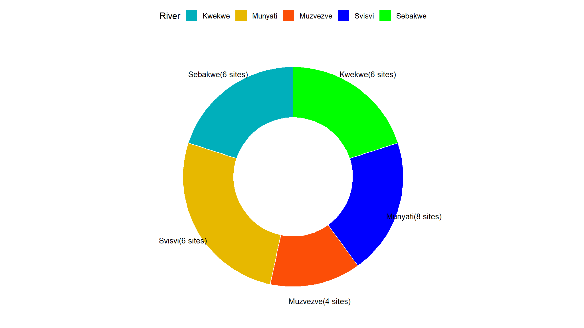
data visualisations of water parameters
(temps+amo) +
  plot_annotation(title = "Average temperature and Ammonia",
                  subtitle = "averaged per River",
                  theme = theme(text = element_text(family = "Asap Condensed"),
                                plot.title = element_text(face = "bold",
                                                          size = rel(1.5))))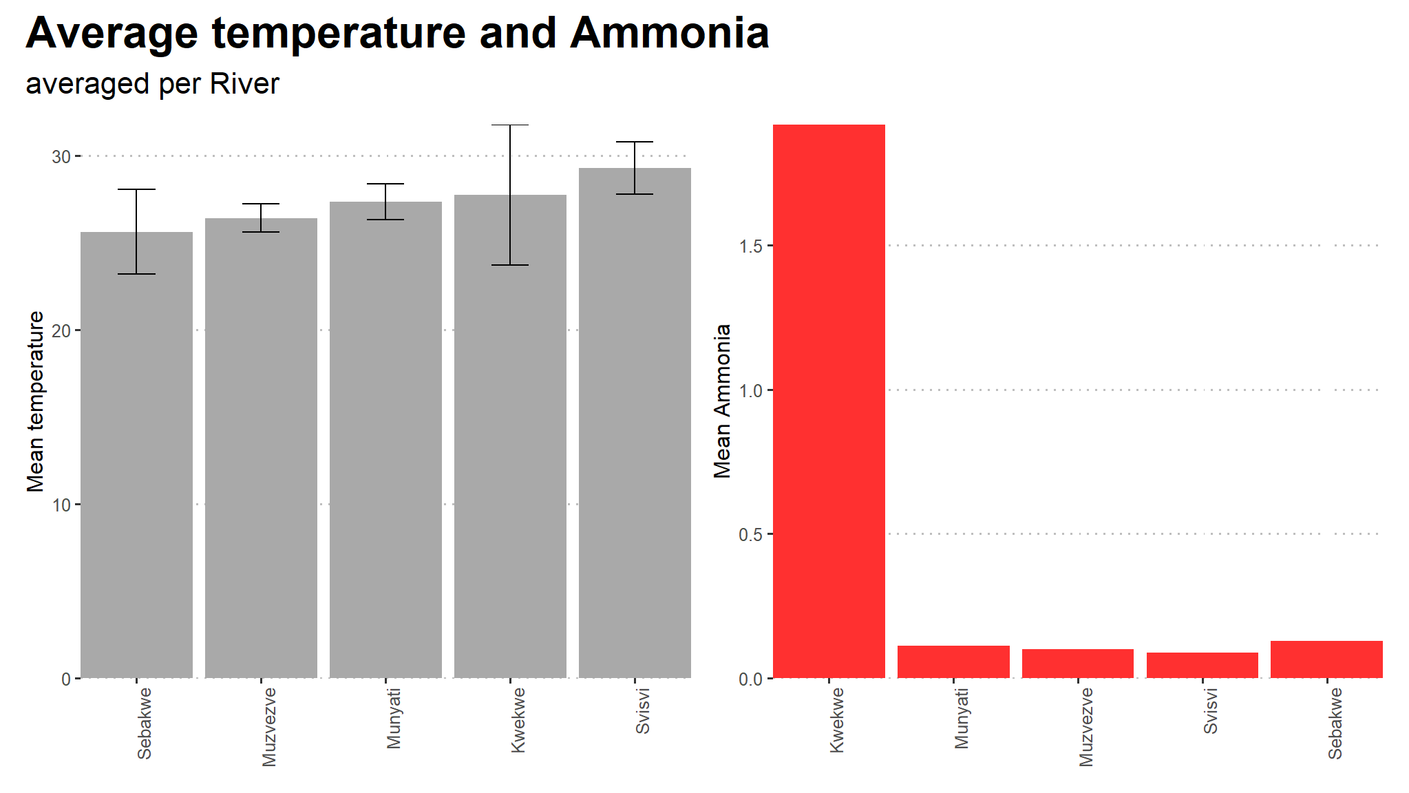
Note
- on average , Kwekwe has the highest level of ammonia as compared to other rivers
- mean temperature is not significantly different between the rivers
(cond+tds) +
  plot_annotation(title = "Average conductivity and total dissolved salts",
                  subtitle = "averaged per River",
                  theme = theme(text = element_text(family = "Asap Condensed"),
                                plot.title = element_text(face = "bold",
                                                          size = rel(1.5))))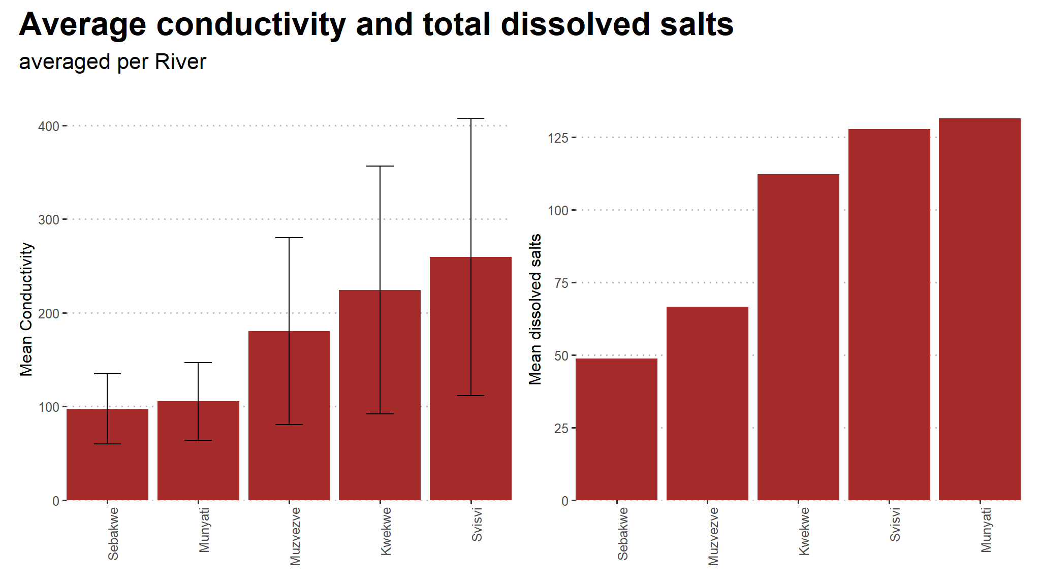
Note
- On average ,
Munyatihas the greatest amount of dissolved salts - on the other hand
Svisvihas greatest amount of conductivity
(phos+cla) +
  plot_annotation(title = "Average phosphates and clarity",
                  subtitle = "averaged per River",
                  theme = theme(text = element_text(family = "Asap Condensed"),
                                plot.title = element_text(face = "bold",
                                                          size = rel(1.5))))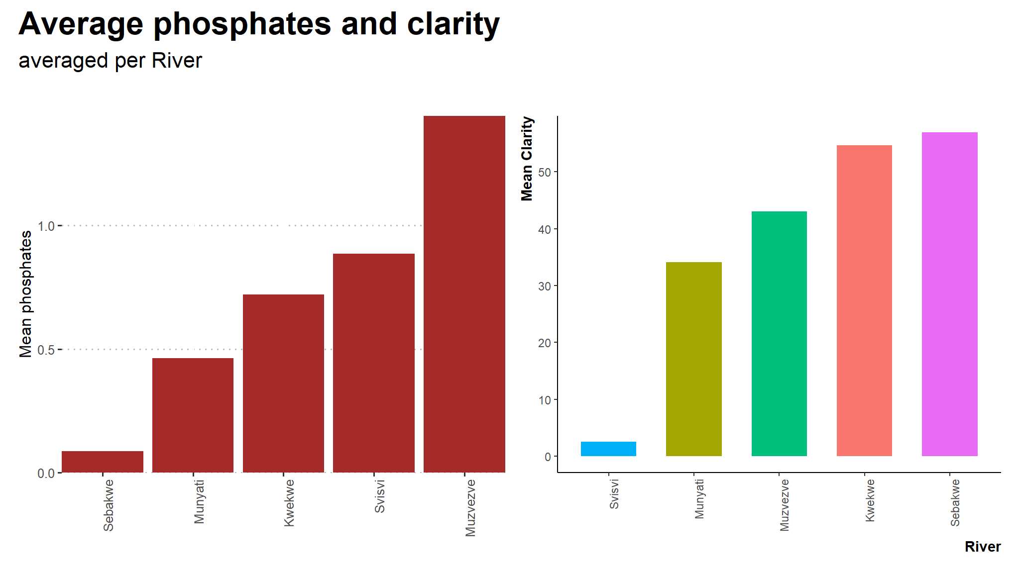
substrates in river
## changing data frame from wide to long
dt2_long<-gather(data2,macroSpecies,number_of_species,Naucoris:Trichoptera)|>
  select(genus,macroSpecies,number_of_species)

dtsum<-dt2_long|>
  group_by(genus)|>
  summarise(total_species=sum(number_of_species))|>
  arrange(desc(total_species))

dtsum<- data1%>%
  mutate(substrate=as.factor(substrate),Stream.order=as.factor(Stream.order))|>
  group_by(River,substrate)|>
  summarise(n=n())|>
  arrange(n)|>
  dplyr::mutate(perc = paste0(sprintf("%4.1f", n/ sum(n) * 100), "%"))

## river and substrate type ###
dt<- data1%>%
  mutate(substrate=as.factor(substrate),
         Stream.order=as.factor(Stream.order))|>
 group_by(River,substrate)|>
    summarise(n=n())|>
  mutate(val=n/sum(n),
         perc=scales::percent(val))

dt |>  ggplot(
  aes(x=River,y=val,fill=substrate))+
  geom_bar(stat="identity",
          position="fill")+
  geom_text(aes(label=perc),
            size=3,
            position=position_stack(vjust=0.5))+
  scale_fill_brewer(palette="set1")+
  theme(axis.text.x = element_text(angle = 45, hjust = 1, vjust = 1),
        legend.position = "top")+
  labs(y="percent substrate",
       fill="substrate type",
       x="River",title="Substrate type by River")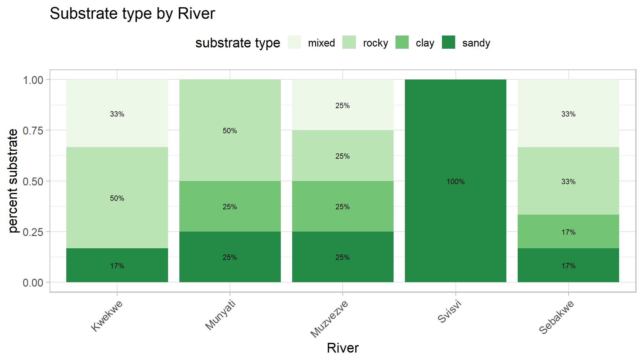
Stream order and macroinvertebrates
dtsum<-dt2_long|>
  group_by(genus,macroSpecies)|>
  summarise(total_species=sum(number_of_species))|>
  arrange(desc(total_species))

dtsum|>
  ggplot(aes(x=reorder(genus,total_species),y=total_species))+
  geom_col() +
  coord_flip()+
  labs(x="Site",y="Total number of macroinvertebrates",
       title="Distribution of macroinvertebrates \n per site")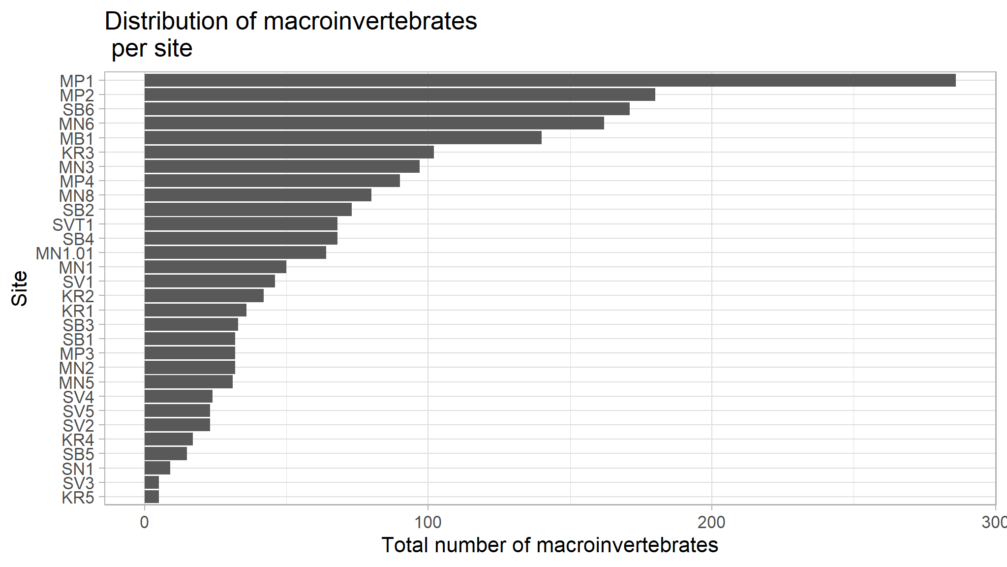
## relative frequencies and abundance
dtsum<- data1%>%
  mutate(substrate=as.factor(substrate),
         Stream.order=as.factor(Stream.order))|>
 group_by(River,Stream.order)|>
    summarise(n=n())|> arrange(n)|>
  dplyr::mutate(perc = paste0(sprintf("%4.1f", n/ sum(n) * 100), "%"))

ggplot(dtsum, aes(x =n, y =River,fill=Stream.order)) +
  geom_col() +
  theme_classic() +
  coord_flip()+
  theme(
    axis.text.y = element_text(size = 14, hjust = 1),
    axis.text.x = element_text(angle = 45, hjust = 1, vjust = 1),
    plot.margin = margin(rep(15, 4))) +
  labs(title="Distribution of River Samples and their Stream order")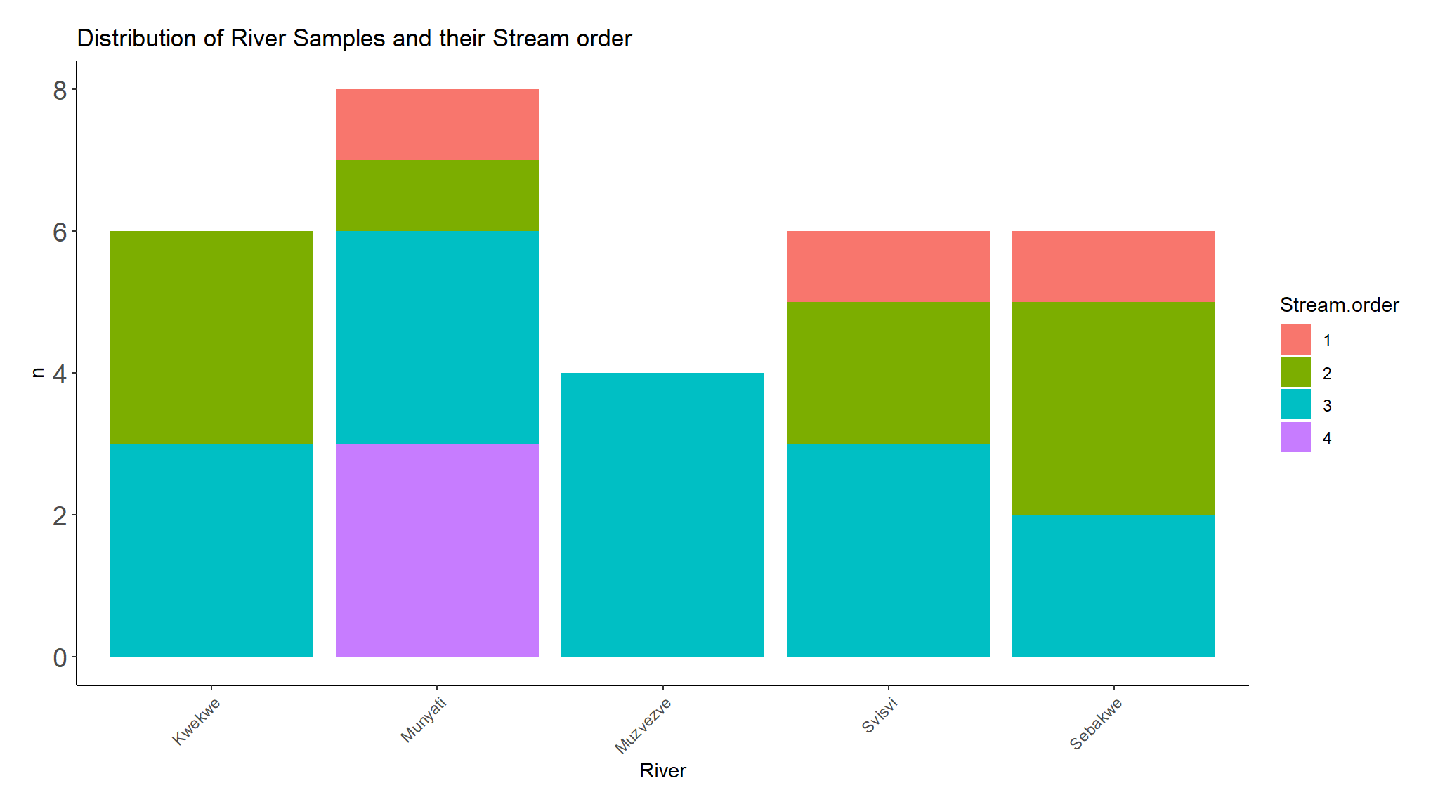
Descriptive statistical Analysis by River
| Characteristic | Kwekwe, N = 6 | Munyati, N = 8 | Muzvezve, N = 4 | Svisvi, N = 6 | Sebakwe, N = 6 | Test Statistic | p-value1 |
|---|---|---|---|---|---|---|---|
| Alpha, Mean (SD) | 11 (6) | 14 (5) | 18 (7) | 8 (2) | 13 (6) | 2.8 | 0.046 |
| DO, Mean (SD) | 6.88 (1.24) | 6.06 (1.48) | 5.70 (1.45) | 7.78 (0.69) | 5.13 (2.47) | 2.5 | 0.065 |
| DO.sat, Mean (SD) | 85 (15) | 76 (18) | 70 (19) | 98 (5) | 68 (23) | 2.9 | 0.042 |
| Clarity, Mean (SD) | 55 (39) | 34 (31) | 43 (42) | 3 (1) | 57 (24) | 3.3 | 0.028 |
| salinity, Mean (SD) | 0.10 (0.05) | 0.06 (0.02) | 0.08 (0.04) | 0.10 (0.08) | 0.03 (0.02) | 2.7 | 0.051 |
| Temperature, Mean (SD) | 27.75 (4.03) | 27.36 (1.01) | 26.43 (0.82) | 29.28 (1.50) | 25.63 (2.43) | 2.1 | 0.11 |
| Ammonia, Mean (SD) | 1.92 (1.28) | 0.11 (0.14) | 0.10 (0.07) | 0.09 (0.05) | 0.13 (0.03) | 12 | <0.001 |
| Phosphates, Mean (SD) | 0.72 (0.49) | 0.46 (0.46) | 1.44 (1.71) | 0.89 (0.72) | 0.09 (0.05) | 2.3 | 0.091 |
| Cond, Mean (SD) | 224 (132) | 106 (41) | 180 (100) | 259 (148) | 97 (37) | 3.3 | 0.026 |
| TDS, Mean (SD) | 112 (66) | 131 (217) | 67 (67) | 128 (74) | 49 (19) | 0.53 | 0.71 |
| Elevation, Mean (SD) | 1,269 (113) | 1,105 (288) | 1,145 (183) | 807 (107) | 1,296 (118) | 6.6 | <0.001 |
| substrate, n / N (%) | 0.063 | ||||||
| mixed | 2 / 6 (33%) | 0 / 8 (0%) | 1 / 4 (25%) | 0 / 6 (0%) | 2 / 6 (33%) | ||
| rocky | 3 / 6 (50%) | 4 / 8 (50%) | 1 / 4 (25%) | 0 / 6 (0%) | 2 / 6 (33%) | ||
| clay | 0 / 6 (0%) | 2 / 8 (25%) | 1 / 4 (25%) | 0 / 6 (0%) | 1 / 6 (17%) | ||
| sandy | 1 / 6 (17%) | 2 / 8 (25%) | 1 / 4 (25%) | 6 / 6 (100%) | 1 / 6 (17%) | ||
| 1 One-way ANOVA; Fisher’s exact test | |||||||
Note
- there is significant differences in mean alpha diversity between the rivers
(p<0.05) - there is also significant difference in mean
ammonia,conductivity, clarity and elevation - though the p-value is small , we would assume there is significant association between
substrate and River
But which rivers actually have different Alpha diversity?
we perform a POST HOC analysis
#>   Tukey multiple comparisons of means
#>     95% family-wise confidence level
#>
#> Fit: aov(formula = Alpha ~ River, data = data1)
#>
#> $River
#>                        diff        lwr        upr     p adj
#> Munyati-Kwekwe     3.541667  -4.881312 11.9646451 0.7315913
#> Muzvezve-Kwekwe    7.166667  -2.900718 17.2340515 0.2552279
#> Svisvi-Kwekwe     -3.333333 -12.337876  5.6712094 0.8113581
#> Sebakwe-Kwekwe     2.333333  -6.671209 11.3378760 0.9393348
#> Muzvezve-Munyati   3.625000  -5.925760 13.1757598 0.7973212
#> Svisvi-Munyati    -6.875000 -15.297978  1.5479784 0.1491607
#> Sebakwe-Munyati   -1.208333  -9.631312  7.2146451 0.9929891
#> Svisvi-Muzvezve  -10.500000 -20.567385 -0.4326152 0.0379058
#> Sebakwe-Muzvezve  -4.833333 -14.900718  5.2340515 0.6271945
#> Sebakwe-Svisvi     5.666667  -3.337876 14.6712094 0.3699209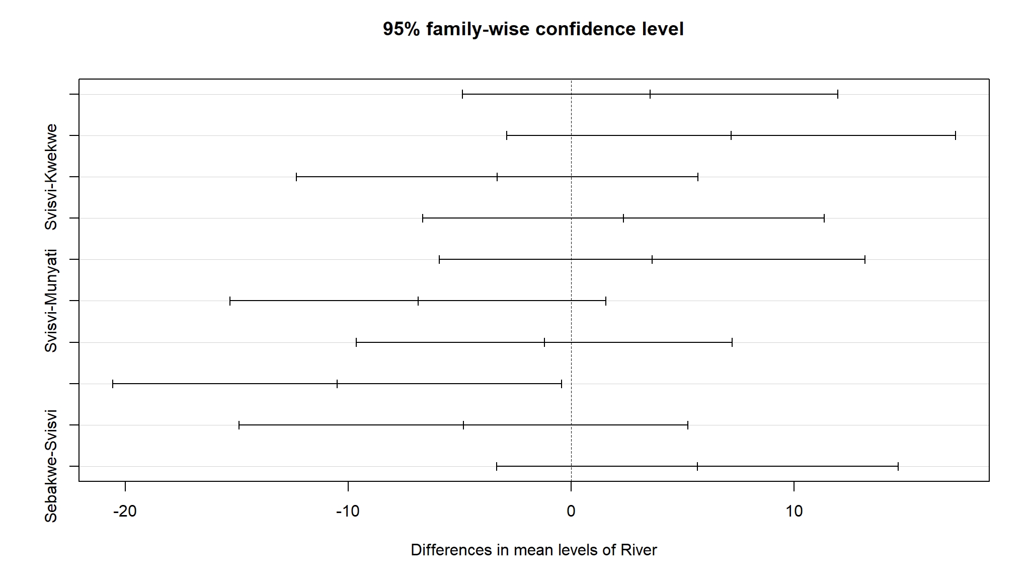
Note
- only Svisvi and Muzvezve have significant mean differences in Alpha diversity
Descriptive statistical analysis by Substrate type
| Characteristic | mixed, N = 51 | rocky, N = 101 | clay, N = 41 | sandy, N = 111 | Test Statistic | p-value2 |
|---|---|---|---|---|---|---|
| Alpha | 13 (4) | 11 (5) | 16 (7) | 12 (7) | 0.69 | 0.57 |
| DO | 6.20 (2.76) | 6.60 (1.26) | 5.45 (1.80) | 6.48 (1.70) | 0.43 | 0.73 |
| DO.sat | 83 (20) | 81 (16) | 68 (24) | 82 (21) | 0.63 | 0.60 |
| Clarity | 44 (19) | 54 (33) | 26 (50) | 24 (32) | 1.6 | 0.21 |
| salinity | 0.07 (0.05) | 0.08 (0.05) | 0.05 (0.03) | 0.08 (0.06) | 0.36 | 0.78 |
| Temperature | 27.50 (3.23) | 26.09 (1.79) | 26.45 (2.30) | 28.76 (2.20) | 2.7 | 0.069 |
| Ammonia | 1.39 (1.70) | 0.40 (0.64) | 0.05 (0.04) | 0.27 (0.58) | 2.5 | 0.078 |
| Phosphates | 0.59 (0.61) | 0.42 (0.45) | 0.41 (0.51) | 0.99 (1.14) | 1.0 | 0.39 |
| Cond | 145 (125) | 181 (107) | 105 (58) | 191 (132) | 0.65 | 0.59 |
| TDS | 72 (63) | 93 (51) | 29 (20) | 149 (183) | 1.2 | 0.34 |
| Elevation | 1,252 (119) | 1,190 (180) | 1,044 (393) | 1,029 (269) | 1.4 | 0.26 |
| River | 0.063 | |||||
| Kwekwe | 2 / 5 (40%) | 3 / 10 (30%) | 0 / 4 (0%) | 1 / 11 (9.1%) | ||
| Munyati | 0 / 5 (0%) | 4 / 10 (40%) | 2 / 4 (50%) | 2 / 11 (18%) | ||
| Muzvezve | 1 / 5 (20%) | 1 / 10 (10%) | 1 / 4 (25%) | 1 / 11 (9.1%) | ||
| Svisvi | 0 / 5 (0%) | 0 / 10 (0%) | 0 / 4 (0%) | 6 / 11 (55%) | ||
| Sebakwe | 2 / 5 (40%) | 2 / 10 (20%) | 1 / 4 (25%) | 1 / 11 (9.1%) | ||
| Stream.order | 0.24 | |||||
| 1 | 0 / 5 (0%) | 0 / 10 (0%) | 1 / 4 (25%) | 2 / 11 (18%) | ||
| 2 | 2 / 5 (40%) | 4 / 10 (40%) | 0 / 4 (0%) | 3 / 11 (27%) | ||
| 3 | 3 / 5 (60%) | 5 / 10 (50%) | 1 / 4 (25%) | 6 / 11 (55%) | ||
| 4 | 0 / 5 (0%) | 1 / 10 (10%) | 2 / 4 (50%) | 0 / 11 (0%) | ||
| 1 Mean (SD); n / N (%) | ||||||
| 2 One-way ANOVA; Fisher’s exact test | ||||||
Note
none of the test outputs is significant enough at 5% level of significance
Correlations between alpha diversity and different water parameters
data1 |>
  select_if(is.numeric) |>
  gather("features","values",-Alpha) |>
  group_by(features) |>
  mutate(coef_dat=round(cor(values,Alpha),2)) |>
  mutate(features=paste(features,' vs Alpha , r= ' ,coef_dat ,sep="")) |>
  ggplot(aes(x=values,y=Alpha,color=features))+
  geom_point(show.legend = F)+
  geom_smooth()+
  facet_wrap(~features,scales="free")+
  ggthemes::scale_color_stata()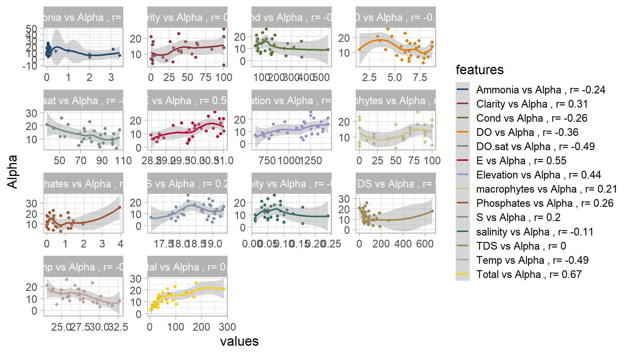
Note
- there happen to be a high degree of negative correlation between
alpha diversity and c(temperature,Dissolved oxygen saturation)whilst there is some significant correlation betweenAlpha diversity and Elevation
Principal component analysis
- prepare the data for
PCA
#subsetting only the numerical variables
pc_data <-data1|>
  select(Alpha,macrophytes,DO.sat,Clarity,salinity,Temp,Ammonia,Phosphates,Cond,TDS,Elevation,DO,site)

pc_data<-column_to_rownames(pc_data,var="site")
#making the PCA dataframe
# NB : can also use prcomp(p, center = TRUE, scale = TRUE)
## Principal component analysis

#same as scale(pc_data) |> prcomp
cor_pca <- prcomp(pc_data, scale = T)
manually calculate eigen values,propotion and cumulative propotion
# eigen values
cor_results <- data.frame(eigen_values = cor_pca$sdev ^ 2)
cor_results |>
    mutate(proportion = eigen_values / sum(eigen_values),
           cumulative = cumsum(proportion))
#>    eigen_values  proportion cumulative
#> 1    3.61943351 0.301619459  0.3016195
#> 2    2.34486631 0.195405525  0.4970250
#> 3    1.70074657 0.141728881  0.6387539
#> 4    1.25065342 0.104221118  0.7429750
#> 5    1.11059667 0.092549722  0.8355247
#> 6    0.75108740 0.062590616  0.8981153
#> 7    0.48820937 0.040684114  0.9387994
#> 8    0.32120028 0.026766690  0.9655661
#> 9    0.25538431 0.021282026  0.9868482
#> 10   0.09492865 0.007910720  0.9947589
#> 11   0.04668138 0.003890115  0.9986490
#> 12 0.01621214 0.001351012 1.0000000summary(cor_pca)
#> Importance of components:
#> PC1 PC2 PC3 PC4 PC5 PC6 PC7
#> Standard deviation 1.9025 1.5313 1.3041 1.1183 1.05385 0.86665 0.69872
#> Proportion of Variance 0.3016 0.1954 0.1417 0.1042 0.09255 0.06259 0.04068
#> Cumulative Proportion 0.3016 0.4970 0.6388 0.7430 0.83552 0.89812 0.93880
#> PC8 PC9 PC10 PC11 PC12
#> Standard deviation 0.56675 0.50536 0.30810 0.21606 0.12733
#> Proportion of Variance 0.02677 0.02128 0.00791 0.00389 0.00135
#> Cumulative Proportion 0.96557 0.98685 0.99476 0.99865 1.00000using factoextra
library(factoextra)

# estimate pca scores by covariate

components <- prcomp(pc_data, scale = TRUE)

# apply rotation

components$rotation <- components$rotation

# show components

components$rotation|>
  as.data.frame()
#>                     PC1          PC2          PC3         PC4         PC5
#> Alpha       -0.35449121 -0.099861865  0.034611711  0.18790555 -0.46343472
#> macrophytes -0.23230742 -0.092419235  0.548808883  0.05226851  0.12074187
#> DO.sat       0.44589849 -0.009195734  0.224887088  0.30018957  0.12908776
#> Clarity     -0.28029176 -0.381657502  0.010384165  0.31668735  0.24755452
#> salinity     0.24173971 -0.514308694 -0.008787703 -0.12921516 -0.17433411
#> Temp         0.29431009  0.264654513 -0.380144332 -0.17037232 -0.03403939
#> Ammonia      0.10928400 -0.218758665 -0.523617522  0.21447741  0.41251633
#> Phosphates   0.01194742 -0.102994483 -0.294317484  0.47150593 -0.60047136
#> Cond         0.28872248 -0.489789925  0.039847584 -0.14116307 -0.10158596
#> TDS          0.01386244 -0.359919212  0.016981856 -0.54622162 -0.12690411
#> Elevation   -0.37989159 -0.253279618 -0.250867727  0.03512616  0.30801738
#> DO           0.39745139 -0.095572209  0.277007128  0.37147576  0.09548333
#>                     PC6         PC7         PC8         PC9         PC10
#> Alpha        0.28166620  0.42228029 -0.39808272 -0.37170706 -0.175865531
#> macrophytes -0.48446951 -0.14559438  0.03116949 -0.46254752  0.317589568
#> DO.sat      -0.04479548  0.21536370 -0.28856902  0.04201020  0.193054265
#> Clarity     -0.30526222 -0.21353368 -0.35832964  0.30406258 -0.487119843
#> salinity     0.18413223 -0.26871710 -0.19197187 -0.27528921  0.221645383
#> Temp        -0.37035133 -0.07870618 -0.62879524 -0.09712516  0.101071591
#> Ammonia     -0.09713152  0.21785145  0.28089682 -0.53855533 -0.142456583
#> Phosphates  -0.37482391 -0.10109928  0.27969256  0.17060108  0.244652854
#> Cond         0.19578007 -0.29303947  0.05169217  0.04862992 -0.116988890
#> TDS         -0.42867332  0.56184694  0.08984046  0.18520043 -0.055715660
#> Elevation    0.20587477  0.13821484 -0.16681026  0.28456362  0.661267540
#> DO           0.07276285  0.38957946  0.03081807  0.17793314  0.009800876
#>                    PC11         PC12
#> Alpha        0.16632006 -0.014207618
#> macrophytes  0.16749334 -0.138718540
#> DO.sat       0.11295599  0.678442518
#> Clarity     -0.12866827  0.024799710
#> salinity    -0.60166250 -0.002640343
#> Temp         0.14943825 -0.296522618
#> Ammonia      0.05009729  0.034839451
#> Phosphates   0.02297821  0.036238312
#> Cond         0.70318702 -0.086679360
#> TDS         -0.04938556  0.090379332
#> Elevation    0.13897252 -0.074904239
#> DO -0.10666523 -0.638673640fviz_screeplot(components, addlabels = TRUE, ylim = c(0, 36))+
labs(title='Figure 11. Proportion of Variance Explained by Individual PCA Components (Dimensions)')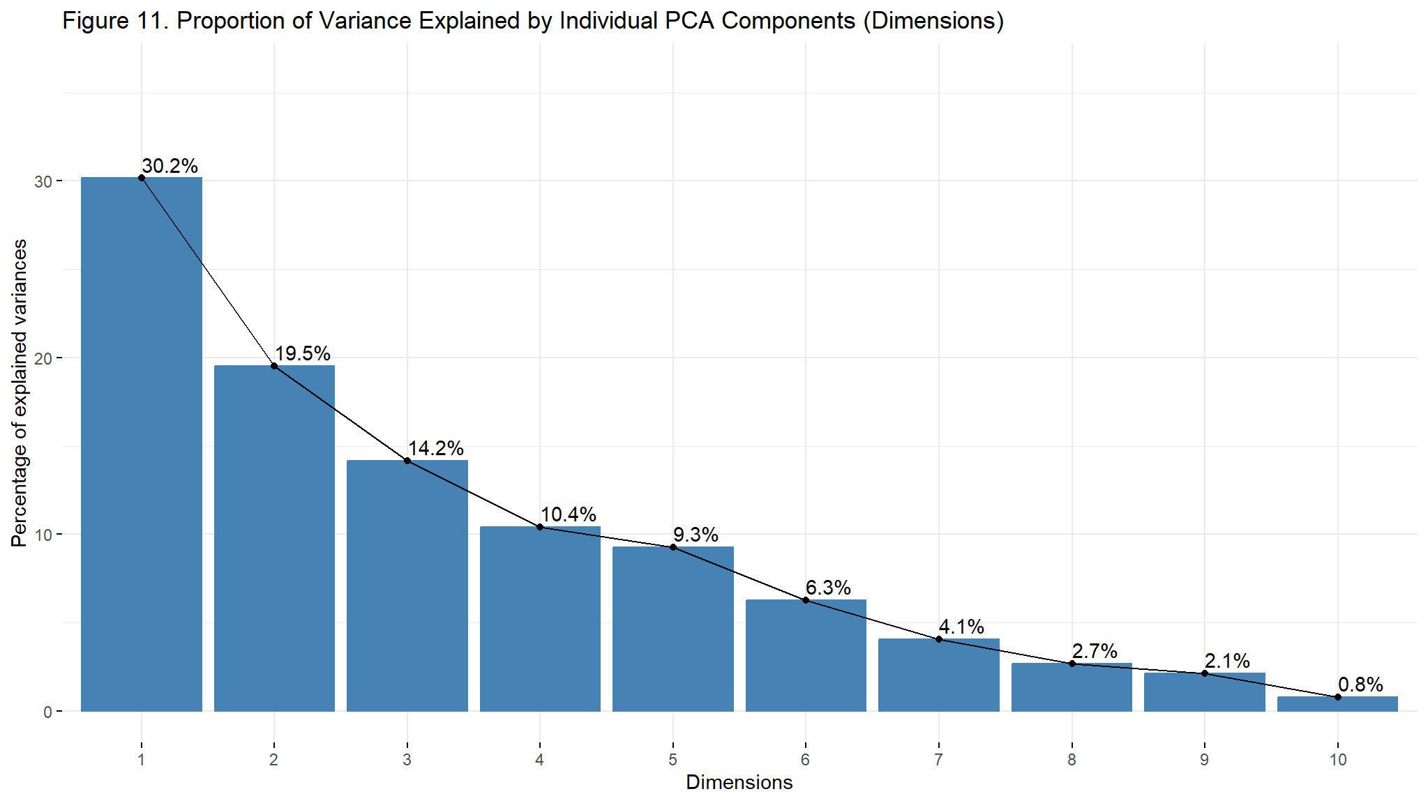
Note
- from the screeplot , the first 4 principal components contain about 84.3% of the variability in the data
- on the other hand the first five components contribute about 83.6% of the variability in the data and small for the subsequent PCs
- thus the first four components are an effective summary of all the variables thus instead of working with all the variables ,we could use the 4 or 5 components for future modeling.
assess variable importance to each if the first 4 components (dim)
v1<-fviz_contrib(components, choice = "var", axes = 1, top = 10, title='Contribution of Variables \n to PCA1')
v2<-fviz_contrib(components, choice = "var", axes = 2, top = 10, title='Contribution of Variables \n to PCA2')
v3<-fviz_contrib(components, choice = "var", axes = 3, top = 10, title='Contribution of Variables \n to PCA3')
v4<-fviz_contrib(components, choice = "var", axes = 4, top = 10, title='Contribution of Variables \n to PCA4')v1|v2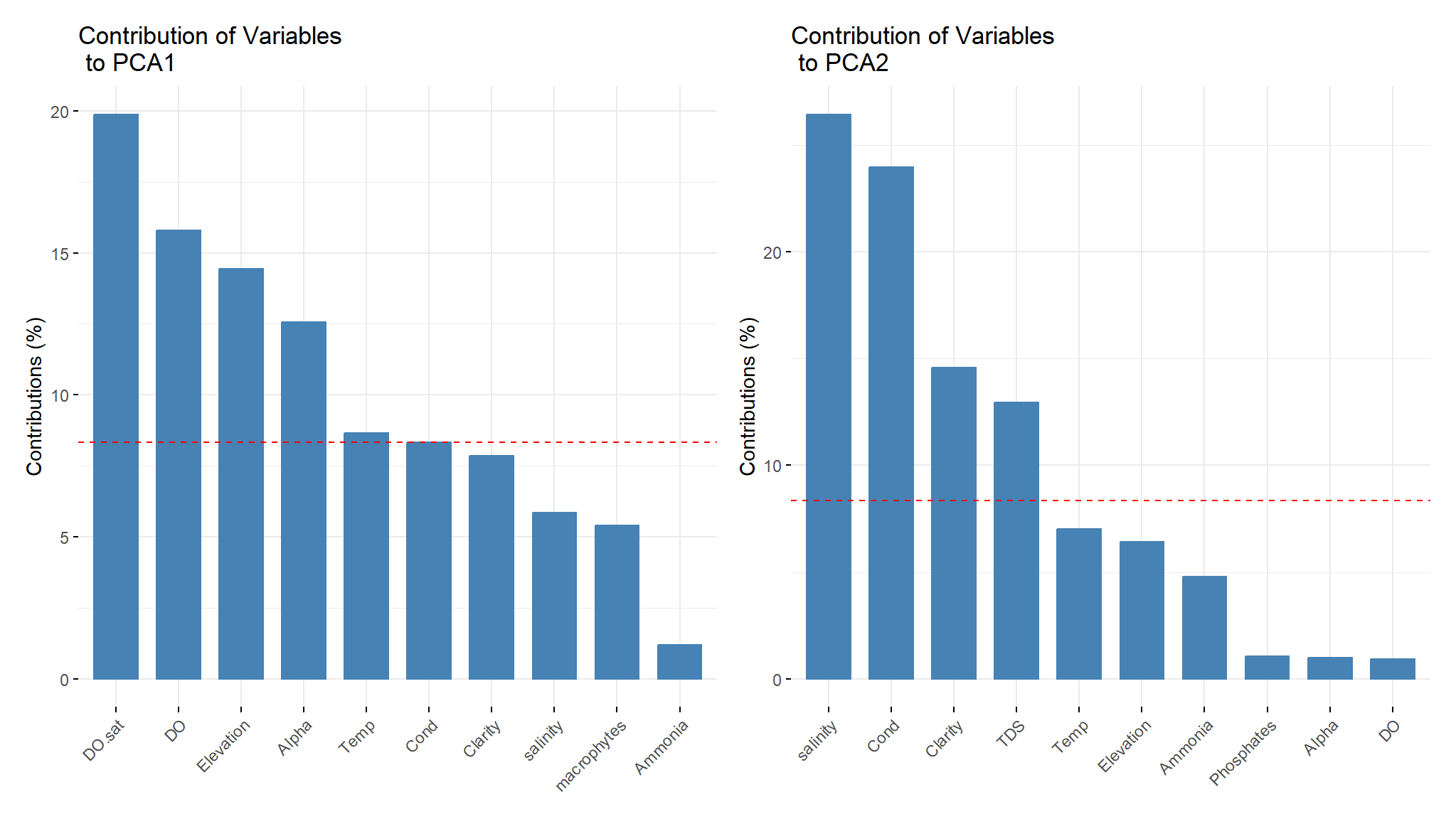
Note
- the red dashed line on the graphs above indicate the expected average contribution . for a certain component , a variable with a contribution exceeding this benchmark is considered as important in contributing to the component .
- from the output Dissolved oxygen saturation, Dissolved oxygen ,Elevetation and temperature contribute the most to first component.
- On the other hand salinity,conductivity ,clarity and Total dissolved salts contribute more to second component.
v3|v4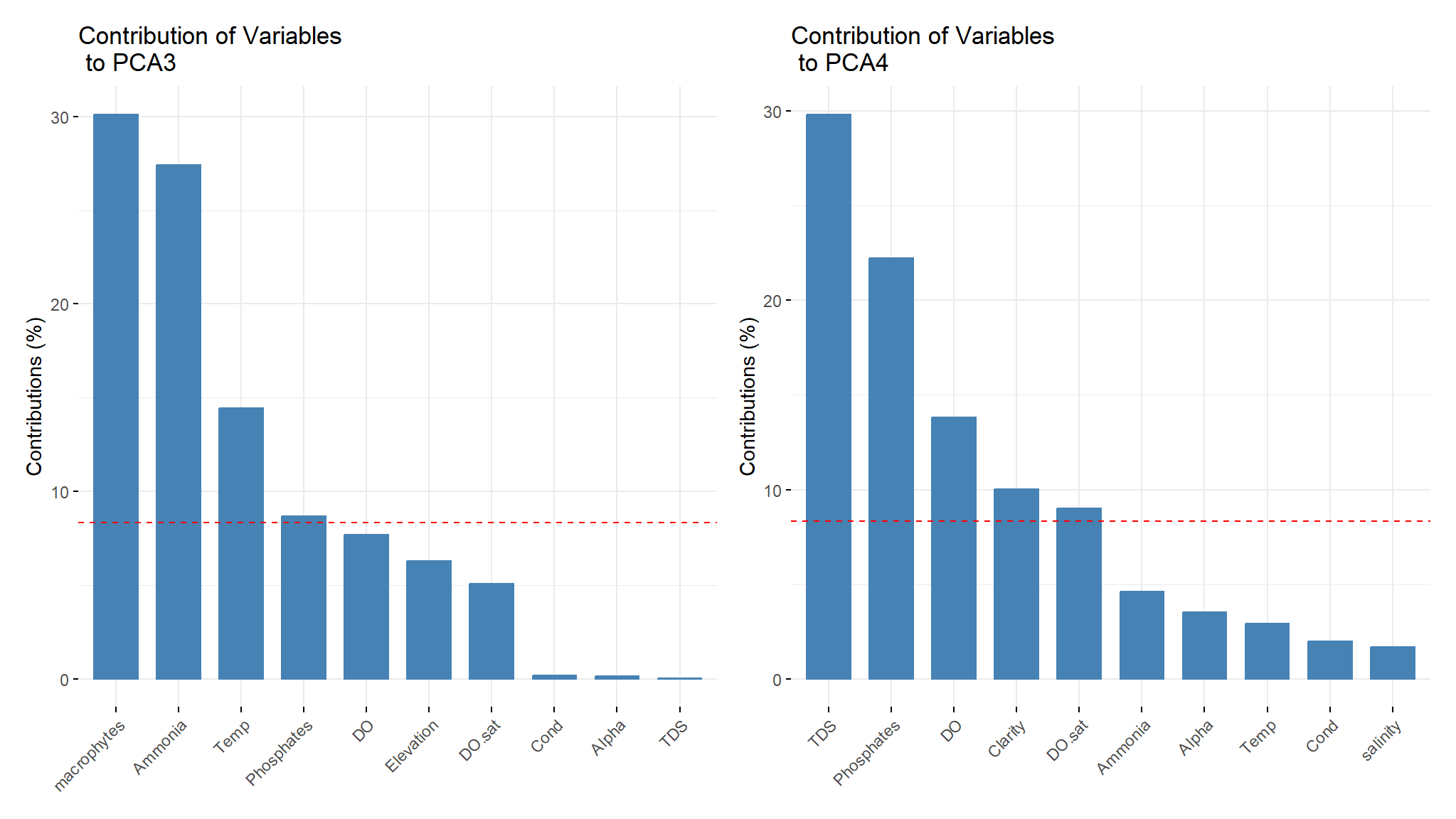
Note
- macrophytes , Ammonia and Temperature contribute significantly on PCA3
Visualizing PCA
The PCA can be visualized by using a variable factor map and an individual factor map or a combination of both maps, called the biplot. The variable plot shows the variables as vectors (arrows). The vectors start at the origin [0,0] and extend to coordinates given by the loading vector. This plot illustrates the contribution of each variable to components and the correlation of each variable.
fviz_pca_var(components, alpha.var = "contrib", col.var = "contrib", # Color by contributions to the PC
             gradient.cols = c("#00AFBB", "#E7B800", "#FC4E07"),
             title = 'Influence of Variables on PCA1 and PCA2', repel = TRUE )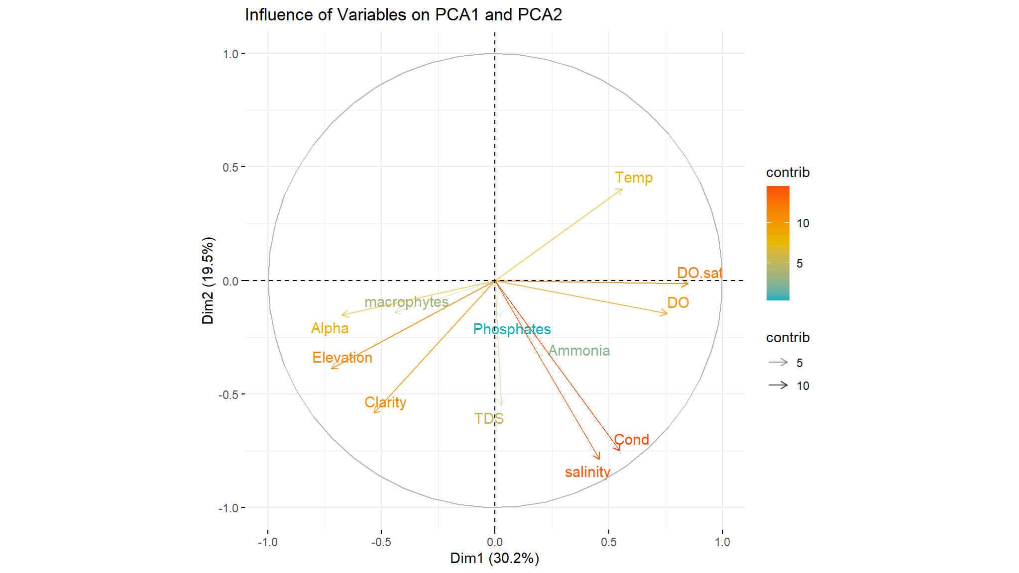
Insight from variables factor map :
The more parallel the arrows (variables) to PC, the more those variables contribute to that PC. thus we note that Dissolved oxygen saturation, Dissolved oxygen and temperature contribute positively to the first PC , Alpha diversity and macrophytes contribute negatively to first component
The longer the arrow, the more variability of this variable is represented by two PC (red arrows).
Correlation between each variable can be defined by the angle between arrows and positively correlated variables are grouped together. A high positive correlation is represented by small-angle differences thus we note that
Alpha diversity ,macrophytes ,Elevation and Clarityare in the same direction hence they are correlated in some way ,
it really make sense since macroinvertebrates feed on macrophytes and they need clear water to survive.
#Biplot of individuals and variables
fviz_pca_biplot(components, repel = TRUE,
                title='Distribution of numeric variables: from PCA1 and PCA2',
                col.var = "#2E9FDF",col.ind = "#696969",)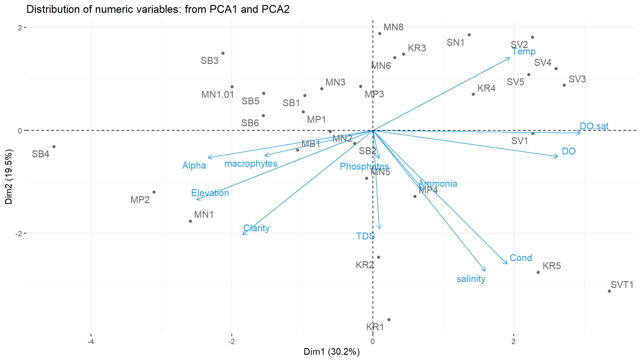
Note
- the plot shows which which sites actually have the highest of the variables pointed to them
- site
MP2 ,MN1 and MB1are high in alpha diversity
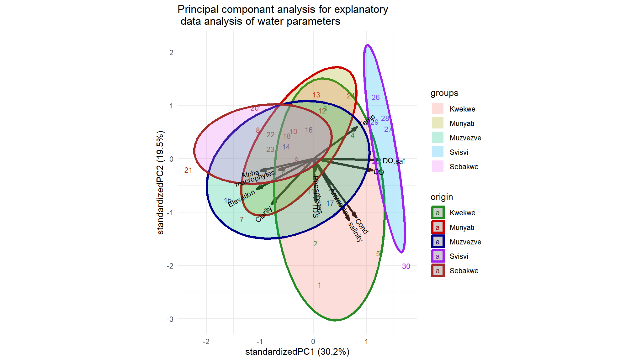
Principal component ellipses
Statistical modeling
- we begin off with a linear regression model
mod_lm<-lm(Alpha~River+DO+Cond+TDS+Clarity+Temp+macrophytes+Ammonia+Phosphates+Elevation+Stream.order+substrate,data=data1)
summary(mod_lm)
#>
#> Call:
#> lm(formula = Alpha ~ River + DO + Cond + TDS + Clarity + Temp +
#>     macrophytes + Ammonia + Phosphates + Elevation + Stream.order +
#>     substrate, data = data1)
#>
#> Residuals:
#>     Min      1Q  Median      3Q     Max
#> -4.8528 -1.2873 -0.0888  1.3829  5.1517
#>
#> Coefficients:
#>                  Estimate Std. Error t value Pr(>|t|)
#> (Intercept)     72.160087  29.454947   2.450  0.03427 *
#> RiverMunyati    -7.984290   4.318036  -1.849  0.09419 .
#> RiverMuzvezve   -7.949404   4.959435  -1.603  0.14004
#> RiverSvisvi    -22.088267   8.649163  -2.554  0.02868 *
#> RiverSebakwe    -8.303602   3.913732  -2.122  0.05986 .
#> DO               0.476949   0.808486   0.590  0.56833
#> Cond            -0.005017   0.010937  -0.459  0.65625
#> TDS             -0.002222   0.010932  -0.203  0.84302
#> Clarity          0.040850   0.045816   0.892  0.39355
#> Temp            -0.983857   0.589829  -1.668  0.12627
#> macrophytes     -0.114893   0.056560  -2.031  0.06965 .
#> Ammonia         -7.878375   2.419128  -3.257  0.00862 **
#> Phosphates       3.367858   1.730696   1.946  0.08028 .
#> Elevation       -0.005399   0.011221  -0.481  0.64076
#> Stream.order2   -9.346333   5.250047  -1.780  0.10539
#> Stream.order3   -9.358622   6.309718  -1.483  0.16884
#> Stream.order4   -7.370862   9.946471  -0.741  0.47570
#> substraterocky  -8.612929   2.763446  -3.117  0.01093 *
#> substrateclay   -6.753207   3.861545  -1.749  0.11089
#> substratesandy  -3.449021   3.380512  -1.020  0.33165
#> ---
#> Signif. codes:  0 '***' 0.001 '**' 0.01 '*' 0.05 '.' 0.1 ' ' 1
#>
#> Residual standard error: 3.596 on 10 degrees of freedom
#> Multiple R-squared:  0.8736, Adjusted R-squared:  0.6335
#> F-statistic: 3.639 on 19 and 10 DF,  p-value: 0.02046
Note
- most variables have negative effects on Alpha diversity based on the
coefficientof the variables substraterocky and ammoniahave coefficients that are statistically significant- the overal model is better than a null model
(p=0.02046) - the amount of variability explained is \(R^2=0.8736 =87\%\) implying a linear model captures the data well
performance::check_model(mod_lm)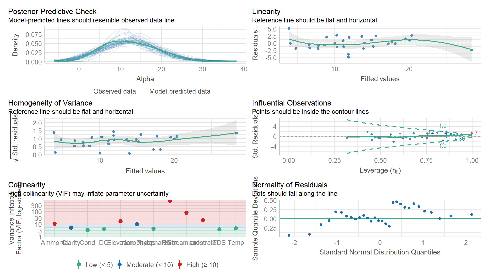
- however from the smoothened scatter plots plotted earlier , it can be noted that some variables are not linear to
Alpha diversityhence the need forgeneralised Additive Models
Generalised Additive models
Briefly, GAMs are effectively a nonparametric form of regression where the \(\beta x_i\) of a linear regression is replaced by a smooth function of the explanatory variables, \(f(x_i)\), and the model becomes:
\[y_i = f(x_i) + \epsilon_i\] where \(y_i\) is the response variable, \(x_i\) is the predictor variable, and \(f\) is the smooth function.
Importantly, given that the smooth function \(f(x_i)\) is non-linear and local, the magnitude of the effect of the explanatory variable can vary over its range, depending on the relationship between the variable and the response.
That is, as opposed to one fixed coefficient \(\beta\), the function \(f\) can continually change over the range of \(x_i\). The degree of smoothness (or wiggliness) of \(f\) is controlled using penalized regression determined automatically in mgcv using a generalized cross-validation (GCV) routine
We can try to build a more appropriate model by fitting the data with a smoothed (non-linear) term. In mgcv::gam(), smooth terms are specified by expressions of the form s(x), where \(x\) is the non-linear predictor variable we want to smooth.
mod_gam1<-mgcv::gam(Alpha~River+s(DO)+s(Cond)+s(TDS)+s(Clarity)+s(Temp)+s(macrophytes)+s(Ammonia)+s(Phosphates)+s(Elevation)+Stream.order+substrate,data=data1,method="REML")
summary(mod_gam1)
#>
#> Family: gaussian
#> Link function: identity
#>
#> Formula:
#> Alpha ~ River + s(DO) + s(Cond) + s(TDS) + s(Clarity) + s(Temp) +
#>     s(macrophytes) + s(Ammonia) + s(Phosphates) + s(Elevation) +
#>     Stream.order + substrate
#>
#> Parametric coefficients:
#>                Estimate Std. Error t value Pr(>|t|)
#> (Intercept)      37.661      7.344   5.128 0.000634 ***
#> RiverMunyati    -10.095      3.766  -2.681 0.025310 *
#> RiverMuzvezve    -8.814      4.176  -2.111 0.064183 .
#> RiverSvisvi     -24.878      7.329  -3.395 0.008014 **
#> RiverSebakwe     -9.678      3.351  -2.888 0.018059 *
#> Stream.order2   -10.335      4.381  -2.359 0.042854 *
#> Stream.order3   -10.342      5.326  -1.942 0.084304 .
#> Stream.order4    -5.466      8.726  -0.626 0.546690
#> substraterocky   -9.764      2.358  -4.141 0.002554 **
#> substrateclay    -9.465      3.452  -2.742 0.022901 *
#> substratesandy   -2.768      2.864  -0.966 0.359326
#> ---
#> Signif. codes:  0 '***' 0.001 '**' 0.01 '*' 0.05 '.' 0.1 ' ' 1
#>
#> Approximate significance of smooth terms:
#>                  edf Ref.df      F p-value
#> s(DO)          1.000   1.00  0.003 0.96083
#> s(Cond)        1.000   1.00  0.081 0.78288
#> s(TDS)         1.000   1.00  0.434 0.52632
#> s(Clarity)     1.000   1.00  2.381 0.15724
#> s(Temp)        1.000   1.00  5.585 0.04237 *
#> s(macrophytes) 1.000   1.00  6.419 0.03204 *
#> s(Ammonia)     1.000   1.00 19.388 0.00171 **
#> s(Phosphates)  2.057   2.46  1.718 0.18961
#> s(Elevation)   1.000   1.00  0.614 0.45344
#> ---
#> Signif. codes:  0 '***' 0.001 '**' 0.01 '*' 0.05 '.' 0.1 ' ' 1
#>
#> R-sq.(adj) =  0.749   Deviance explained = 92.3%
#> -REML =   42.6  Scale est. = 8.8445    n = 30
Caution
We’ll start with the effective degrees of freedom[^lme4], or edf. In typical OLS regression the model degrees of freedom is equivalent to the number of features/terms in the model. This is not so straightforward with a GAM due to the smoothing process and the penalized regression estimation procedure, something that will be discussed more later[^edfinit]. In this situation, we are still trying to minimize the residual sums of squares, but we also have a built-in penalty for ‘wiggliness’ of the fit, where in general we try to strike a balance between an undersmoothed fit and an oversmoothed fit. The default p-value for the test is based on the effective degrees of freedom and the rank \(r\) of the covariance matrix for the coefficients for a particular smooth, so here, conceptually, it is the p-value associated with the \(F(r, n-edf)\).
Note
- looking at the output ,variables that have
effective degrees of freedom(edf=1)generally have been reduced to linear effect - we can remove the smooth functions
s()for variables that haveedf=1
mod_gam1<-mgcv::gam(Alpha~River+DO+Cond+TDS+Clarity+Temp+macrophytes+Ammonia+s(Phosphates)+Elevation+Stream.order+substrate,data=data1,method="REML")
summary(mod_gam1)
#>
#> Family: gaussian
#> Link function: identity
#>
#> Formula:
#> Alpha ~ River + DO + Cond + TDS + Clarity + Temp + macrophytes +
#>     Ammonia + s(Phosphates) + Elevation + Stream.order + substrate
#>
#> Parametric coefficients:
#>                  Estimate Std. Error t value Pr(>|t|)
#> (Intercept)     87.446880  25.231425   3.466  0.00716 **
#> RiverMunyati   -10.095091   3.765690  -2.681  0.02531 *
#> RiverMuzvezve   -8.814419   4.175921  -2.111  0.06418 .
#> RiverSvisvi    -24.878492   7.328794  -3.395  0.00801 **
#> RiverSebakwe    -9.677819   3.351070  -2.888  0.01806 *
#> DO               0.035880   0.710315   0.051  0.96082
#> Cond            -0.002635   0.009282  -0.284  0.78291
#> TDS             -0.006156   0.009340  -0.659  0.52643
#> Clarity          0.065323   0.042337   1.543  0.15745
#> Temp            -1.185668   0.501690  -2.363  0.04254 *
#> macrophytes     -0.119475   0.047155  -2.534  0.03219 *
#> Ammonia         -9.246293   2.099816  -4.403  0.00174 **
#> Elevation       -0.007359   0.009393  -0.784  0.45356
#> Stream.order2  -10.334564   4.381227  -2.359  0.04285 *
#> Stream.order3  -10.341613   5.326404  -1.942  0.08430 .
#> Stream.order4   -5.466459   8.726297  -0.626  0.54668
#> substraterocky  -9.764217   2.358169  -4.141  0.00255 **
#> substrateclay   -9.464739   3.451659  -2.742  0.02290 *
#> substratesandy  -2.767558   2.864216  -0.966  0.35932
#> ---
#> Signif. codes:  0 '***' 0.001 '**' 0.01 '*' 0.05 '.' 0.1 ' ' 1
#>
#> Approximate significance of smooth terms:
#>                 edf Ref.df     F p-value
#> s(Phosphates) 2.057   2.46 3.512  0.0531 .
#> ---
#> Signif. codes:  0 '***' 0.001 '**' 0.01 '*' 0.05 '.' 0.1 ' ' 1
#>
#> R-sq.(adj) =  0.749   Deviance explained = 92.3%
#> -REML = 66.01 Scale est. = 8.8445 n = 30- First ,from a statistical standpoint we come with almost the same results as the linear model
- now
ammonia , macrophytes and Temperaturehave statistically significant effect on Alpha diversity - moreover , our
deviance explained value has increased to 92.3\%showing a better improvement and convincing us to take nonlinear model more seriously - most variables generally have negative impact on
Alpha diversity, for instance decreasing ammonia increasesalpha diversityand the result is statistically significant. Ammonia is bad for species diversity. - we would also expect an increase in water clarity to increase species diversity as well
Test for a better model
anova(mod_lm,mod_gam1,test="Chisq")
#> Analysis of Variance Table
#>
#> Model 1: Alpha ~ River + DO + Cond + TDS + Clarity + Temp + macrophytes +
#>     Ammonia + Phosphates + Elevation + Stream.order + substrate
#> Model 2: Alpha ~ River + DO + Cond + TDS + Clarity + Temp + macrophytes +
#>     Ammonia + s(Phosphates) + Elevation + Stream.order + substrate
#>    Res.Df     RSS     Df Sum of Sq Pr(>Chi)
#> 1 10.0000 129.337
#> 2  8.9431  79.097 1.0569     50.24  0.01879 *
#> ---
#> Signif. codes:  0 '***' 0.001 '**' 0.01 '*' 0.05 '.' 0.1 ' ' 1
Note
- interesting , not that we couldn`t have assumed as such already but now we have additional statistical evidence to suggest that incorporating nonlinear relationships of the features improves the model.
- the
Pr(>Chi)value is less than0.05indicating that incorporating nonlinear aspect of the variables is important