library(tidyverse)
library(knitr)
library(gtsummary)
library(ggpubr)
library(RColorBrewer)
library(lemon)
library(paletteer)
library(survival)
library(survminer)
library(cowplot)
library(rms)
library(car)
library(patchwork)


options("encoding" = "UTF-8")
knitr::opts_chunk$set(echo = TRUE, message = FALSE, warning = FALSE)

list("style_number-arg:big.mark" = "") %>%
set_gtsummary_theme()Predicting job retention
survival analysis
jobs
statistics
Library Setup
Survival analysis in Job retention prediction
The methodology for predicting job retention will be based on the approach of survival analysis, for which the main variable of interest is the (expected) time to some event. In addition, for each observation we have a status variable, taking value 1 if the event happened at the end of the corresponding time period, or 0 otherwise. Latter observations are called censored: it means that we observed them for the whole time period without the event, but we admit that this event can happen for them in the future (after the period of observation), so the time to event for them will be censored on the right and will be denoted as observation time+. If no observations were censored, we could use standard regression models for continuous responses to predict time to event or models for binary classification to predict the probability of event during some preliminary specified period of time (for example, one year after beginning of observation). Besides taking censoring into account, in comparison with these models survival analysis have several advantages
One of the functions used in survival analysis, the hazard function, helps to understand the mechanism of failure (in our case the mechanism of retention) and how it changes over the survival time (period of followup). Moreover, we can predict patterns in outcome (retention behavior) over time for individual subjects.
Conceptual framework of survival analysis
In our study the event is a left, i.e. A binary variable indicating whether or not the individual had left their job as at the last follow-up. Our target variable is time to event (T) - The month of the last follow-up.
We will assume that T is a continuous random variable with probability density function f(t) and cumulative distribution function \(F(t) = P(T < t)\), giving the probability that the event has occurred by time t. In survival analysis the statistical model for time to event (T) is usually defined with the complement of cumulative density function , called a survival function S(t). Survival function is the probability that an individual survives from the time origin to a specified time t or, equivalently, that the event has not occurred by time t and will (may) occur after it. In our analysis it will be the probability that a user remains active from the start of his/her subscription to a specified time point t (or probability that he/she churn some time after t): \[S(t) = P(T>t) = 1-F(t)=\int_t^\infty f(t)\]
Survival function is non-increasing with t and equals 1 at t = 0 .
Another important term in survival analysis is hazard h(t)
- the probability that an individual who is still observed at time t has an event in small interval after t: \[h(t)=\lim_{u \to 0}\frac{P(t<T<t+u | T>t)}{u} = \frac{f(t)}{S(t)}=-\frac{d}{dt}logS(t)\] Hazard will characterize the intensity of churn over time, i.e. a rate of churn per unit of time. As the width of the interval (u) goes to zero, we obtain an instantaneous rate of churn for some specific time point.
The numerator in the first part of the above expression is the conditional probability that the churn will occur in the small interval after t ([t, t+u)) given that it has not occurred before, and the denominator is the width of the interval (u). The second part of the formula says that the hazard rate of churn at time t equals the density of churns at t, divided by the probability of membership lasting to that point in time without churning. In addition, it can be proven that h(t) equals the minus slope of the log of the survival function. The latter gives us the formula \[S(t) = exp(-\int_0^t h(v)dv)\]
At last, the area under the curve for hazard h(t) is a cumulative hazard function (H(t)): \[H(t) = \int_0^t h(v)dv = -logS(t)\] It presents the sum of the risks you face going from duration 0 to t [@rodriguez_chapter_2007]. From the last equation we have \[S(t) = exp(-H(t))\]
Therefore, knowing any one of the functions S(t), H(t), or h(t) allows one to derive the other two functions. These three functions are different ways of describing the same distribution for the time to event.
One of the problems in survival analysis is that the form of the true population survival distribution function S(t) is almost always unknown. As a consequence, we should use some estimate for it. If there is no censoring, we can use empirical distribution function of time to event, \(F_n(t)\), to nonparametrically estimate survival as \(S_n(t) = 1 - F_n(t) = [\text{number of }T_i > t]/n\) [@harrell_regression_2015]. With censoring taking place we can use either other nonparametric estimates (the most frequently used here are Kaplan–Meier product-limit estimator and Nelson-Aalen estimator) or parametrically estimate the survival function (it means that we should specify a functional form for S(t) and estimate its unknown parameters). Parametric models give more precise and smooth estimates for survival, hazard and cumulative hazard, allows to easily compute quantiles for time to event and to predict it, but they require accurate specification of distribution function.
Prediction models in survival analysis
Survival regression models
All survival regression models can be divided into two main groups, depending on their assumptions of the nature of covariates’ effects, namely: accelerated failure time and proportional hazard models.
1) Accelerated failure time (AFT) models:
Predictors act multiplicatively on the failure time or additively on the log failure time: \[logT = X\beta + \sigma\epsilon \Rightarrow T = exp(X\beta)T_0\] where X is a \(n*m\) matrix of m characteristics for n individuals (may include an intercept), \(\beta\) - a vector of m coefficients (weights), \(epsilon\) - an error term with some prespecified distribution \(\psi\) (see below) or estimated non-parametrically (rarely used), \(\sigma\) - a scale parameter, \(T_0 = exp(\sigma\epsilon)\) [@rodriguez_chapter_2007; @harrell_regression_2015].
The value of \(exp(X\beta) = \gamma\) is called an accelerator factor, because the effect of a predictor in AFT models is to alter the rate at which a subject proceeds along the time axis (i.e., to accelerate the time to failure) [@harrell_regression_2015]. For example, the failure time for the i-th individual with the j-th characteristic by one unit higher than for the k-th subject (all other things being equal) will be \(exp(\beta_j)\) times the failure time of the k-th subject.
Using AFT models, we can easily predict different representations of the individual survival distribution – of course, if such nature of variables effect on time is typical for the field of study. In addition, AFT models are usually parametric and require accurate assumptions about errors distribution (\(\psi\)) (for details see @abdul-fatawu_accelerated_2020 and @harrell_regression_2015). We do not plan using them in this study.
2) Proportional hazards (PH) models:
While AFT models assumes that predictors have a multiplicative effect on the time to event and additive effect for the log time to event, proportional hazards models assumes the same for the hazard and log hazard, accordingly [@rodriguez_chapter_2007]: \[h(t|X) = h_0(t)exp(X\beta) \Rightarrow log(h(t|X)) = log(h_0(t)) + X\beta\] where \(h_0(t)\) is the baseline hazard function (when all predictors equal zero), \(X\) - matrix of features (not including a constant!), \(\beta\) - regression coefficients (weights). Here \(exp(x_i^`\beta)\) is the relative risk associated with the set of characteristics x_i for the i-th individual in comparison with the risk of an individual with all characteristics equal zero. So in contrast to AFT models, the hazard is positively related to the risk component, \(exp(X\beta)\).
The alternative way to specify a PH regression is to add a constant to feature matrix, such that: \[h(t|X) = exp([C|X]\beta)\] then baseline hazard will be estimated as \(h_0(t)=exp(\beta_0)\), where \(\beta_0\) is the weight for the intercept.
It is important to emphasize that the relative risk does not depend on time, i.e. it is constant in time for the same pair of values of any feature, so hazards are proportional independent of time.
The same holds for cumulative hazards [@rodriguez_chapter_2007]: \[H(t|X) = H_0(t)exp(X\beta)\]
The corresponding survival function will be [@rodriguez_chapter_2007]: \[S(t|X) = S_0(t)^{exp(X\beta)}\] where \(S_0(t)\) is the baseline survival function. Thus, the effect of the set of characteristics \(x_i\) for the i-th individual on the survivor function is to raise it to a power given by the relative risk \(exp(x_i^`\beta)\).
We can use some specific distribution for the baseline survival or hazard function – and then we get a parametric PH model, or do not make such assumptions about the baseline functions – and then get a semi-parametric PH model, often called a Cox PH model after its author.
Survival Analysis for Modeling Singular Events Over Time
The job retention data set shows the results of a study of around 3,800 individuals employed in various fields of employment over a one-year period. At the beginning of the study, the individuals were asked to rate their sentiment towards their job. These individuals were then followed up monthly for a year to determine if they were still working in the same job or had left their job for a substantially different job. If an individual was not successfully followed up in a given month, they were no longer followed up for the remainder of the study period.
Data description
gender: The gender of the individual studiedfield: The field of employment that they worked in at the beginning of the studylevel: The level of the position in their organization at the beginning of the study—Low,MediumorHighsentiment: The sentiment score reported on a scale of 1 to 10 at the beginning of the study, with 1 indicating extremely negative sentiment and 10 indicating extremely positive sentimentleft: A binary variable indicating whether or not the individual had left their job as at the last follow-upmonth: The month of the last follow-up
glimpse to the data
job_retention <- read.csv("job_retention.csv")
head(job_retention)
#>   gender                  field  level sentiment intention left month
#> 1      M      Public/Government   High         3         8    1     1
#> 2      F                Finance    Low         8         4    0    12
#> 3      M Education and Training Medium         7         7    1     5
#> 4      M                Finance    Low         8         4    0    12
#> 5      M                Finance   High         7         6    1     1
#> 6      F                 Health Medium         6        10    1     2
Explanatory analysis
retention by gender and level
plot_data<-job_retention |>
  group_by(gender,left,level) |>
  summarise(value=n()) |>
  mutate(lbl=value/sum(value),
         set="count") |>
  mutate(left=as.factor(left)) |>
  mutate(left=ifelse(left==1,"yes","no")) |>
  rename(group=level)

plot_data |>
  ggplot() +
  geom_bar(aes(x=left, y=value, fill=gender),
           stat = "identity",
           position = position_dodge(0.8), color = "white") +
  geom_text(aes(x=left, y=y, label=lbl, group=gender),
            plot_data %>% mutate(y = value + 0.01, lbl = round(value,3)),
            position = position_dodge(0.8), stat = "identity",
            size = 4, fontface = "bold") +
  facet_rep_grid(set ~ group, repeat.tick.labels = TRUE, switch = "y") +
  scale_y_continuous(expand = c(0,0,0,0.01)) +
  ggthemes::scale_fill_tableau()+
  labs(x="", y="", fill="", title="retention status by level and gender", color="") +
  ggthemes::theme_tufte() +
  theme(legend.position = "top",
        plot.title = element_text(face = "bold", hjust = 0.5),
        axis.ticks.x = element_blank(),
        strip.text = element_text(size = 12, face = "bold"),
        axis.line = element_line(size = .2, color = "grey20"),
        axis.text.x = element_text(size = 12, face = "bold", color = "black"),
        strip.background = element_rect(fill = NA),
        strip.placement = "outside",
        panel.spacing.y=unit(1, "lines"))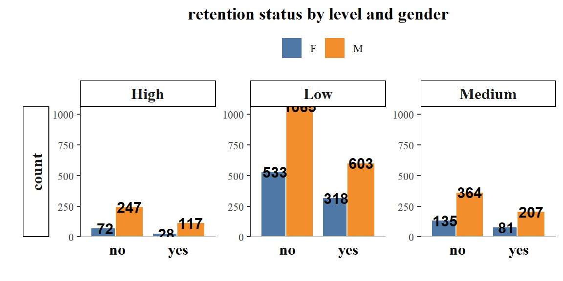
more retention was seen from males a with lower job levels.
Doing survival analysis
# create survival object with event as 'left' and time as 'month'
retention <- Surv(event = job_retention$left,
                  time = job_retention$month)

# view unique values of retention
unique(retention)
#>  [1]  1  12+  5   2   3   6   8   4   8+  4+ 11  10   9   7+  5+  3+  7   9+ 11+
#> [20] 12  10+  6+  2+  1+
We can see that our survival object records the month at which the individual had left their job if they are recorded as having done so in the data set. If not, the object records the last month at which there was a record of the individual, appended with a ‘+’ to indicate that this was the last record available.
The survfit() function allows us to calculate Kaplan-Meier estimates of survival for different groups in the data so that we can compare them. We can do this using our usual formula notation but using a survival object as the outcome. Let’s take a look at survival by gender.
Descriptive statistics and survival analysis
Kaplan-Meier survival curve for the employess are presented below:
srvfit <- survfit(Surv(month, left) ~ 1, job_retention)

p1 <- ggsurvplot(srvfit, size = 1.2,
                 palette = "#006666", conf.int = FALSE,
           ggtheme = theme_minimal() +
             theme(plot.title = element_text(face = "bold")),
           title = "Probability of retention (= survival probability)",
           xlab = "Time from recruitment into study",
           ylab = "Probability of retention",
           legend = "none", censor = FALSE)

p1 <- p1$plot +
  scale_x_continuous(expand = c(0, 0), breaks = seq(0, 12, 1),
                     labels = seq(0, 12, 1),
                     limits = c(0, 820)) +
  scale_y_continuous(expand = c(0, 0), breaks = seq(0,1,0.2),
                     labels = scales::percent_format(accuracy = 1)) +
  theme_classic() +
  theme(legend.position = "none",
        plot.title = element_text(face = "bold"),
        panel.grid.major = element_line(size = .2, colour = "grey90"),
        panel.grid.minor = element_line(size = .2, colour = "grey90"))

p1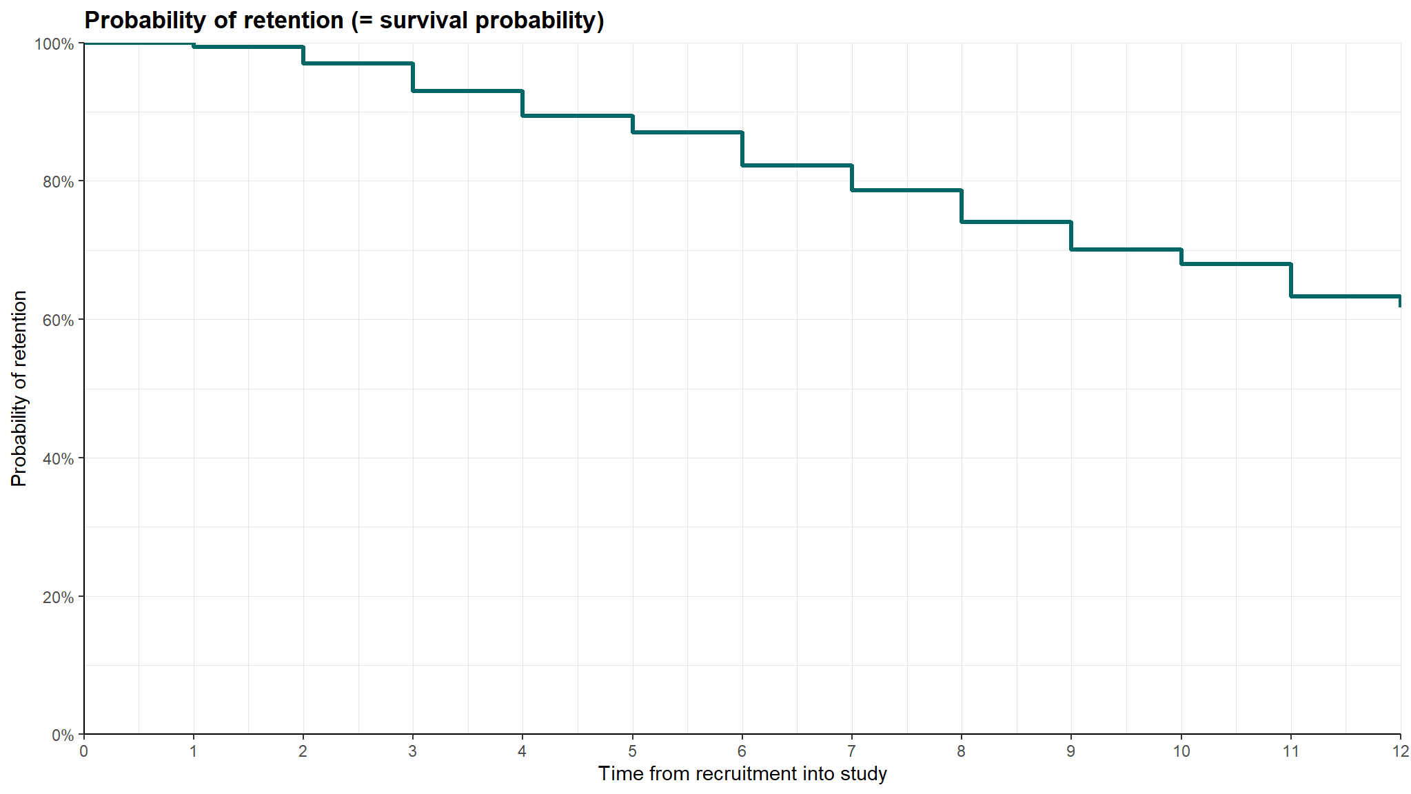
retention by gender
# kaplan-meier estimates of survival by gender
kmestimate_gender <- survival::survfit(
  formula = Surv(event = left, time = month) ~ gender,
  data = job_retention
)

summary(kmestimate_gender)
#> Call: survfit(formula = Surv(event = left, time = month) ~ gender,
#>     data = job_retention)
#>
#>                 gender=F
#>  time n.risk n.event survival std.err lower 95% CI upper 95% CI
#>     1   1167       7    0.994 0.00226        0.990        0.998
#>     2   1140      24    0.973 0.00477        0.964        0.982
#>     3   1102      45    0.933 0.00739        0.919        0.948
#>     4   1044      45    0.893 0.00919        0.875        0.911
#>     5    987      30    0.866 0.01016        0.846        0.886
#>     6    940      51    0.819 0.01154        0.797        0.842
#>     7    882      43    0.779 0.01248        0.755        0.804
#>     8    830      47    0.735 0.01333        0.709        0.762
#>     9    770      40    0.697 0.01394        0.670        0.725
#>    10    718      21    0.676 0.01422        0.649        0.705
#>    11    687      57    0.620 0.01486        0.592        0.650
#>    12    621      17    0.603 0.01501        0.575        0.633
#>
#>                 gender=M
#>  time n.risk n.event survival std.err lower 95% CI upper 95% CI
#>     1   2603      17    0.993 0.00158        0.990        0.997
#>     2   2559      66    0.968 0.00347        0.961        0.975
#>     3   2473     100    0.929 0.00508        0.919        0.939
#>     4   2360      86    0.895 0.00607        0.883        0.907
#>     5   2253      56    0.873 0.00660        0.860        0.886
#>     6   2171     120    0.824 0.00756        0.810        0.839
#>     7   2029      85    0.790 0.00812        0.774        0.806
#>     8   1916     114    0.743 0.00875        0.726        0.760
#>     9   1782      96    0.703 0.00918        0.685        0.721
#>    10   1661      50    0.682 0.00938        0.664        0.700
#>    11   1590     101    0.638 0.00972        0.620        0.658
#>    12   1460      36    0.623 0.00983        0.604        0.642
We can see that the n.risk, n.event and survival columns for each group correspond to the \(n_i\), \(l_i\) and \(S_i\) in our formula above and that the confidence intervals for each survival rate are given. This can be very useful if we wish to illustrate a likely effect of a given input variable on survival likelihood.
plt_df <- job_retention %>%
  mutate(left=ifelse(left==1,"yes","no"))%>%
  group_by(gender,left) %>%
  tally() %>%
  ungroup() %>%
  mutate(pct = n/sum(n)*100,
         lbl = sprintf("%.1f%%", pct))

qbs<-plt_df %>%
 ggplot() +
  aes(x = fct_reorder(gender,pct),y=pct,fill=left) +
 geom_col() +
  geom_text(aes(x = gender, y = pct, label = lbl),
            color = "blue", fontface = "bold") +
  labs(title = "employee sentiment", y = "", x = "") +
  coord_flip()+
  ggthemes::scale_fill_tableau() +
  ggthemes::theme_tufte() +
  theme(legend.position = "bottom",
        plot.title = element_text(face = "bold"),
        axis.text.x = element_text(size = 12),
        axis.ticks.x = element_blank())
srvfit <- survfit(Surv(month, left) ~ gender, job_retention)
qbd <- ggsurvplot(srvfit,
pval = T,
palette = paletteer_d("ggthemes::Tableau_10")[1:length(levels(factor(job_retention$gender)))],
size = 1.2, conf.int = FALSE,
legend.labs = levels(job_retention$gender),
legend.title = "",
ggtheme = theme_minimal() + theme(plot.title = element_text(face = "bold")),
title = "Probability of retention",
xlab = "Time from the first recruit",
ylab = "Probability of retention",
legend = "bottom", censor = FALSE)
qbd<-qbd$plot+
theme_cleantable()qbd+qbs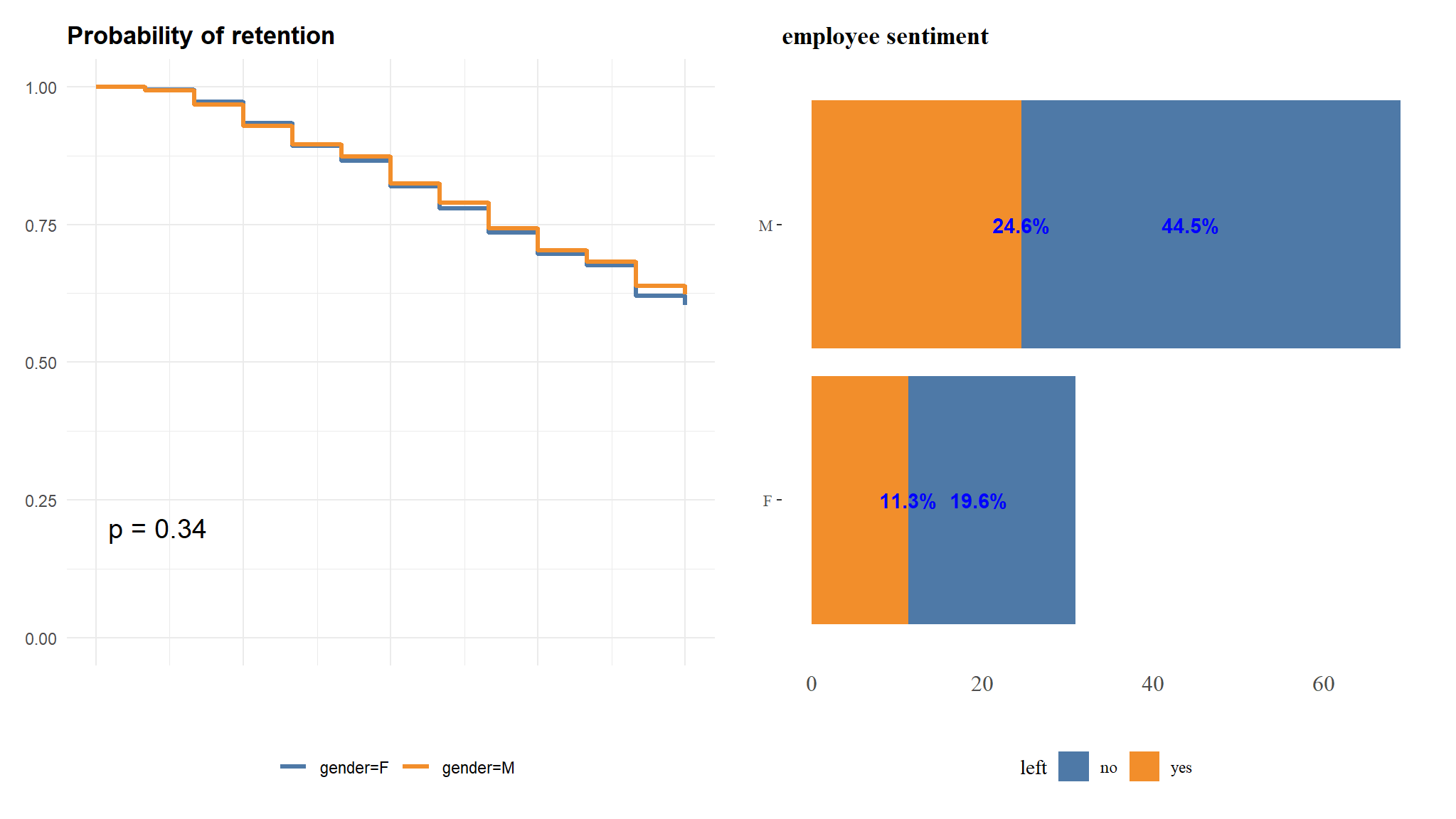
though there is more retention in males than females , there is no significant difference in their retention time.
Let’s imagine that we wish to determine if the sentiment of the individual had an impact on survival likelihood. We can divide our population into two (or more) groups based on their sentiment and compare their survival rates.
without categorizing
plt_df <- job_retention %>%
  mutate(sentiment=as.factor(sentiment)) |>
  group_by(sentiment) %>%
  tally() %>%
  ungroup() %>%
  mutate(pct = n/sum(n)*100,
         lbl = sprintf("%.1f%%", pct))

qb1<-plt_df %>%
 ggplot() +
  aes(x = fct_reorder(sentiment,pct),y=pct) +
  geom_bar(aes(fill = sentiment),stat="identity") +
  geom_text(aes(x = sentiment, y = pct, label = lbl),
            color = "blue", fontface = "bold") +
  labs(title = "employee sentiment", y = "", x = "") +
  coord_flip()+
  ggthemes::scale_fill_tableau() +
  ggthemes::theme_tufte() +
  theme(legend.position = "none",
        plot.title = element_text(face = "bold"),
        axis.text.x = element_text(size = 12),
        axis.ticks.x = element_blank())
srvfit <- survfit(Surv(month, left) ~ sentiment, job_retention)
qb2 <- ggsurvplot(srvfit,
pval = T,
palette = paletteer_d("ggthemes::Tableau_10")[1:length(levels(factor(job_retention$sentiment)))],
size = 1.2, conf.int = FALSE,
legend.labs = levels(job_retention$sentiment),
legend.title = "",
ggtheme = theme_minimal() + theme(plot.title = element_text(face = "bold")),
title = "Probability of retention",
xlab = "Time from the first recruit",
ylab = "Probability of retention",
legend = "bottom", censor = FALSE)
qb2<-qb2$plot(qbd+qbs)/(qb1+qb2)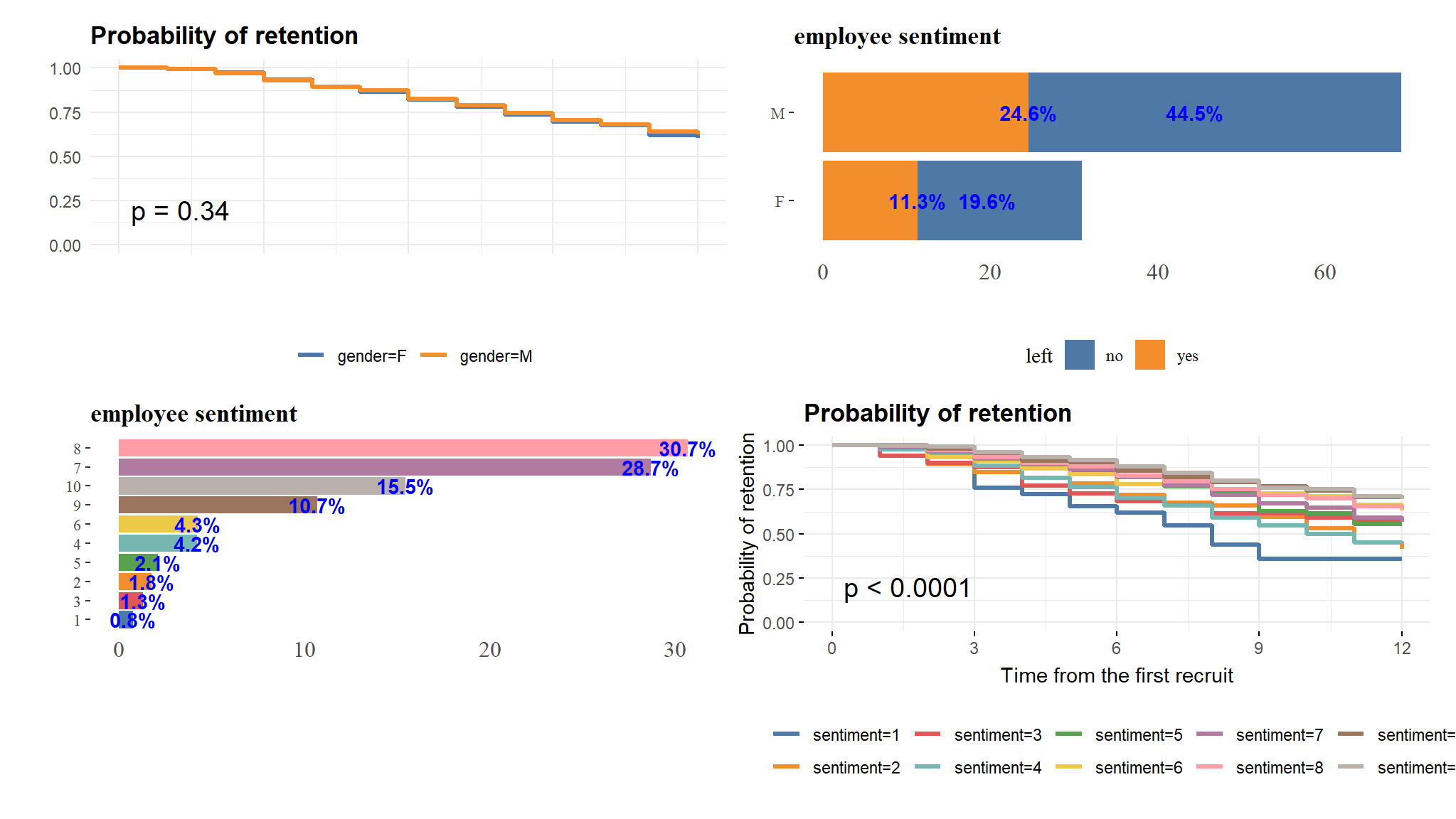
the above is rather hard to read so we might need to categorise the sentiments
# create a new field to define high sentiment (>= 7)
job_retention <-job_retention |>
  mutate(sent_cat = case_when(sentiment >= 7~"High",
                                        between(sentiment,4,6)~"Moderate",
                                        sentiment<=3~"Low"))
# generate survival rates by sentiment category
kmestimate_sentimentcat <- survival::survfit(
formula = Surv(event = left, time = month) ~ sent_cat,
data = job_retention
)
summary(kmestimate_sentimentcat)
#> Call: survfit(formula = Surv(event = left, time = month) ~ sent_cat,
#> data = job_retention)
#>
#> sent_cat=High
#> time n.risk n.event survival std.err lower 95% CI upper 95% CI
#> 1 3225 15 0.995 0.00120 0.993 0.998
#> 2 3167 62 0.976 0.00272 0.971 0.981
#> 3 3075 120 0.938 0.00429 0.929 0.946
#> 4 2932 102 0.905 0.00522 0.895 0.915
#> 5 2802 65 0.884 0.00571 0.873 0.895
#> 6 2700 144 0.837 0.00662 0.824 0.850
#> 7 2532 110 0.801 0.00718 0.787 0.815
#> 8 2389 140 0.754 0.00778 0.739 0.769
#> 9 2222 112 0.716 0.00818 0.700 0.732
#> 10 2077 56 0.696 0.00835 0.680 0.713
#> 11 1994 134 0.650 0.00871 0.633 0.667
#> 12 1827 45 0.634 0.00882 0.617 0.651
#>
#> sent_cat=Low
#> time n.risk n.event survival std.err lower 95% CI upper 95% CI
#> 1 145 3 0.979 0.0118 0.956 1.000
#> 2 139 12 0.895 0.0257 0.846 0.947
#> 3 127 8 0.838 0.0309 0.780 0.901
#> 4 117 8 0.781 0.0348 0.716 0.852
#> 5 109 6 0.738 0.0370 0.669 0.814
#> 6 102 7 0.687 0.0391 0.615 0.769
#> 7 94 6 0.644 0.0405 0.569 0.728
#> 8 86 6 0.599 0.0416 0.522 0.686
#> 9 77 6 0.552 0.0425 0.475 0.642
#> 10 71 5 0.513 0.0429 0.436 0.605
#> 11 66 6 0.466 0.0430 0.389 0.559
#> 12 58 2 0.450 0.0430 0.373 0.543
#>
#> sent_cat=Moderate
#> time n.risk n.event survival std.err lower 95% CI upper 95% CI
#> 1 400 6 0.985 0.00608 0.973 0.997
#> 2 393 16 0.945 0.01142 0.923 0.968
#> 3 373 17 0.902 0.01493 0.873 0.932
#> 4 355 21 0.848 0.01802 0.814 0.885
#> 5 329 15 0.810 0.01978 0.772 0.850
#> 6 309 20 0.757 0.02169 0.716 0.801
#> 7 285 12 0.725 0.02265 0.682 0.771
#> 8 271 15 0.685 0.02365 0.641 0.733
#> 9 253 18 0.637 0.02460 0.590 0.687
#> 10 231 10 0.609 0.02503 0.562 0.660
#> 11 217 18 0.559 0.02563 0.510 0.611
#> 12 196 6 0.541 0.02578 0.493 0.594plt_df <- job_retention %>%
mutate(left=ifelse(left==1,"Yes","No"))%>%
group_by(sent_cat,left) %>%
tally() %>%
ungroup() %>%
mutate(pct = n/sum(n)*100,
lbl = sprintf("%.1f%%", pct))
q1<-plt_df %>%
ggplot() +
aes(x = sent_cat,y=pct,fill=left) +
geom_col() +
geom_text(aes(x = sent_cat, y = pct, label = lbl),
color = "blue", fontface = "bold") +
labs(title = "sentiment category", y = "", x = "") +
ggthemes::scale_fill_fivethirtyeight() +
ggthemes::theme_tufte() +
theme(legend.position = "bottom",
plot.title = element_text(face = "bold"),
axis.text.x = element_text(size = 12),
axis.ticks.x = element_blank())srvfit <- survfit(Surv(month, left) ~ sent_cat, job_retention)
q2 <- ggsurvplot(srvfit,
pval = T,
palette = paletteer_d("ggsci::light_blue_material")[seq(2,10,2)],
size = 1.2, conf.int = FALSE,
legend.labs = levels(job_retention$sent_cat),
legend.title = "",
ggtheme = theme_minimal() + theme(plot.title = element_text(face = "bold")),
title = "Probability of retention",
xlab = "Time from recruitment",
ylab = "Probability of retention",
legend = "bottom", censor = FALSE)
q2<-q2$plotq1+q2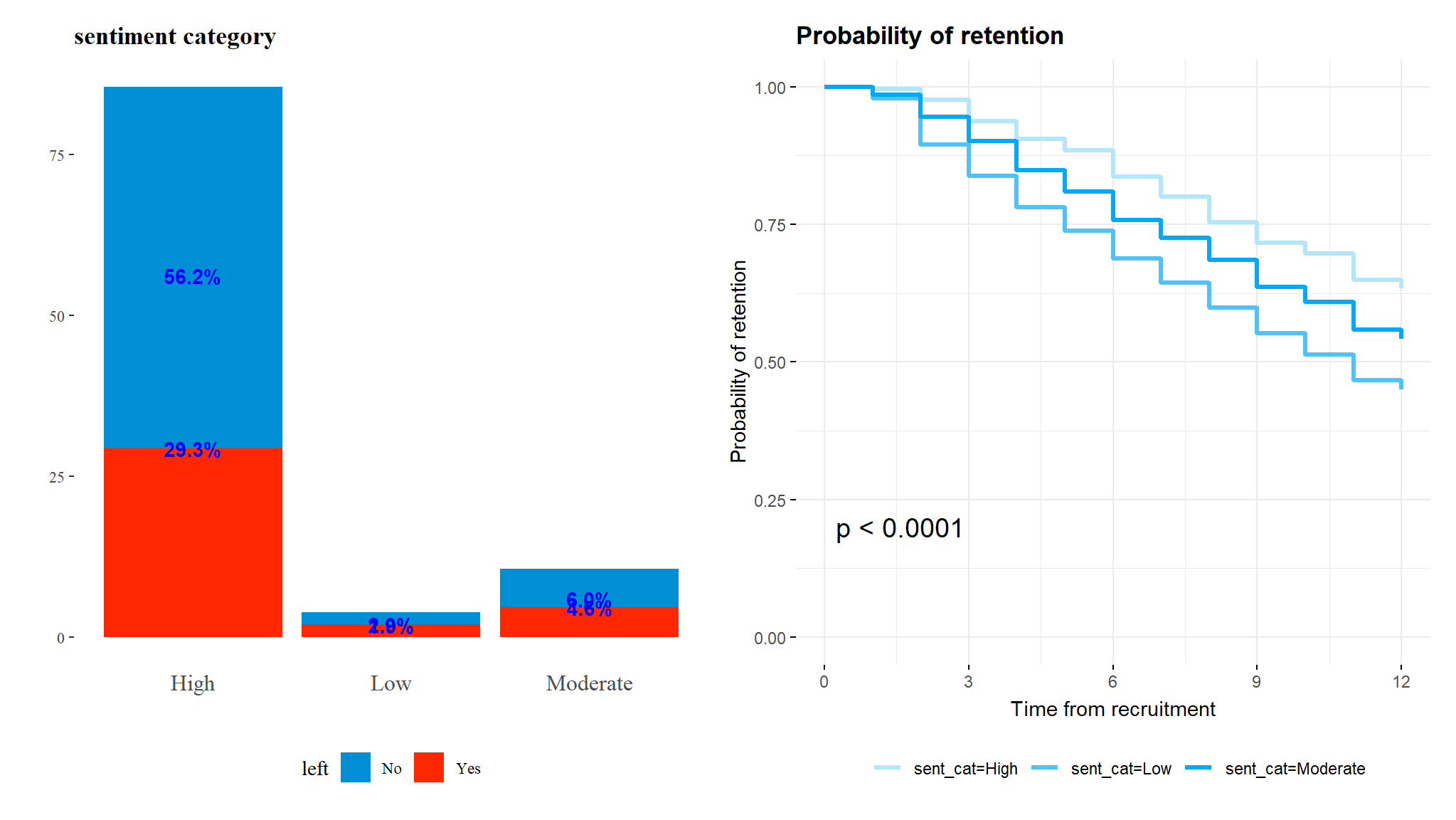
We can see that survival seems to consistently trend higher for those with high sentiment towards their jobs and the differences in survival times is statistically significant.
retention by field
plt_df <- job_retention %>%
  group_by(field) %>%
  tally() %>%
  ungroup() %>%
  mutate(pct = n/sum(n)*100,
         lbl = sprintf("%.0f%%", pct),
         lbl = ifelse(lbl == "0%", "<1%", lbl))

p1<-plt_df %>%
 ggplot() +
  aes(x = fct_reorder(field,pct),y=pct) +
  geom_bar(aes(fill = field),stat="identity") +
  geom_text(aes(x = field, y = pct, label = lbl),
            color = "blue", fontface = "bold") +
  labs(title = "field", y = "proportion(%)", x = "") +
  scale_fill_manual(values = c(paletteer_d("ggthemes::Tableau_10")[1:6])) +
  ggthemes::theme_tufte() +
  theme(legend.position = "none",
        axis.text.x = element_text(angle = 45, hjust = 1),
        plot.title = element_text(face = "bold"),

        axis.ticks.x = element_blank())
srvfit <- survfit(Surv(month, left) ~ field, job_retention)

p2 <- ggsurvplot(srvfit,
                 palette = paletteer_d("ggthemes::Tableau_10")[1:length(levels(factor(job_retention$field)))],
                 size = 1.2, conf.int = FALSE,
                 legend.labs = levels(job_retention$field),
                 legend.title = "",
                 ggtheme = theme_minimal() + theme(plot.title = element_text(face = "bold")),
                 title = "Probability of retention by field",
                 xlab = "Time from recruitment ",
                 ylab = "Probability of retention",
                 legend = "bottom", censor = FALSE,
                 pval=T)


p2<-p2$plotp1+p2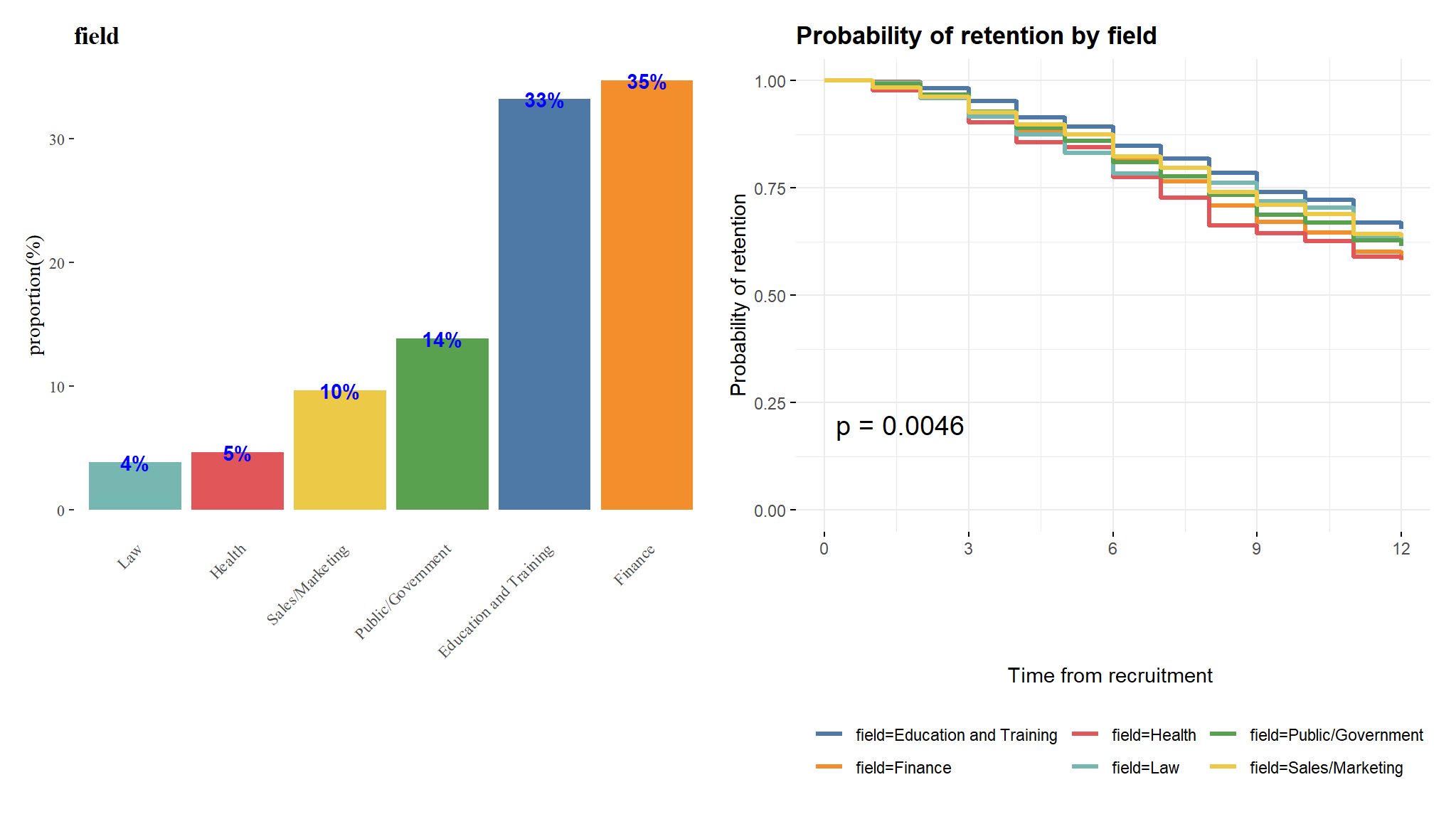
This confirms that the survival difference between the job fields is statistically significant and provides a highly intuitive visualization of the effect of field on retention throughout the period of study.
Cox proportional hazard regression models
Let’s imagine that we have a survival outcome that we are modeling for a population over a time \(t\), and we are interested in how a set of input variables \(x_1, x_2, \dots, x_p\) influences that survival outcome. Given that our survival outcome is a binary variable, we can model survival at any time \(t\) as a binary logistic regression. We define \(h(t)\) as the proportion who have not survived at time \(t\), called the hazard function, and based on our work in Chapter @ref(bin-log-reg):
\[ h(t) = h_0(t)e^{\beta_1x_1 + \beta_2x_2 + \dots + \beta_px_p} \] where \(h_0(t)\) is a base or intercept hazard at time \(t\), and \(\beta_i\) is the coefficient associated with \(x_i\) .
Now let’s imagine we are comparing the hazard for two different individuals \(A\) and \(B\) from our population. We make an assumption that our hazard curves \(h^A(t)\) for individual \(A\) and \(h^B(t)\) for individual \(B\) are always proportional to each other and never cross—this is called the proportional hazard assumption. Under this assumption, we can conclude that
\[ \begin{aligned} \frac{h^B(t)}{h^A(t)} &= \frac{h_0(t)e^{\beta_1x_1^B + \beta_2x_2^B + \dots + \beta_px_p^B}}{h_0(t)e^{\beta_1x_1^A + \beta_2x_2^A + \dots + \beta_px_p^A}} \\ &= e^{\beta_1(x_1^B-x_1^A) + \beta_2(x_2^B-x_2^A) + \dots \beta_p(x_p^B-x_p^A)} \end{aligned} \]
Note that there is no \(t\) in our final equation. The important observation here is that the hazard for person B relative to person A is constant and independent of time. This allows us to take a complicating factor out of our model. It means we can model the effect of input variables on the hazard without needing to account for changes over times, making this model very similar in interpretation to a standard binomial regression model.
Running a Cox proportional hazard regression model
A Cox proportional hazard model can be run using the coxph() function in the survival package, with the outcome as a survival object. Let’s model our survival against the input variables gender, field, level and sentiment.
# run cox model against survival outcome
cox_model <- survival::coxph(
  formula = Surv(event = left, time = month) ~ gender +
    field + level + sentiment,
  data = job_retention
)

summary(cox_model)
#> Call:
#> survival::coxph(formula = Surv(event = left, time = month) ~
#>     gender + field + level + sentiment, data = job_retention)
#>
#>   n= 3770, number of events= 1354
#>
#>                            coef exp(coef) se(coef)      z Pr(>|z|)
#> genderM                -0.04548   0.95553  0.05886 -0.773 0.439647
#> fieldFinance            0.22334   1.25025  0.06681  3.343 0.000829 ***
#> fieldHealth             0.27830   1.32089  0.12890  2.159 0.030849 *
#> fieldLaw                0.10532   1.11107  0.14515  0.726 0.468086
#> fieldPublic/Government  0.11499   1.12186  0.08899  1.292 0.196277
#> fieldSales/Marketing    0.08776   1.09173  0.10211  0.859 0.390082
#> levelLow                0.14813   1.15967  0.09000  1.646 0.099799 .
#> levelMedium             0.17666   1.19323  0.10203  1.732 0.083362 .
#> sentiment              -0.11756   0.88909  0.01397 -8.415  < 2e-16 ***
#> ---
#> Signif. codes:  0 '***' 0.001 '**' 0.01 '*' 0.05 '.' 0.1 ' ' 1
#>
#>                        exp(coef) exp(-coef) lower .95 upper .95
#> genderM                   0.9555     1.0465    0.8514    1.0724
#> fieldFinance              1.2502     0.7998    1.0968    1.4252
#> fieldHealth               1.3209     0.7571    1.0260    1.7005
#> fieldLaw                  1.1111     0.9000    0.8360    1.4767
#> fieldPublic/Government    1.1219     0.8914    0.9423    1.3356
#> fieldSales/Marketing      1.0917     0.9160    0.8937    1.3336
#> levelLow                  1.1597     0.8623    0.9721    1.3834
#> levelMedium               1.1932     0.8381    0.9770    1.4574
#> sentiment                 0.8891     1.1248    0.8651    0.9138
#>
#> Concordance= 0.578  (se = 0.008 )
#> Likelihood ratio test= 89.18  on 9 df,   p=2e-15
#> Wald test            = 94.95  on 9 df,   p=<2e-16
#> Score (logrank) test = 95.31  on 9 df,   p=<2e-16
The model returns the following1
Coefficients for each input variable and their p-values. Here we can conclude that working in Finance or Health is associated with a significantly greater likelihood of leaving over the period studied, and that higher sentiment is associated with a significantly lower likelihood of leaving.
Relative odds ratios associated with each input variable. For example, a single extra point in sentiment reduces the odds of leaving by ~11%. A single less point increases the odds of leaving by ~12%. Confidence intervals for the coefficients are also provided.
Three statistical tests on the null hypothesis that the coefficients are zero. This null hypothesis is rejected by all three tests which can be interpreted as meaning that the model is significant.
Importantly, as well as statistically validating that sentiment has a significant effect on retention, our Cox model has allowed us to control for possible mediating variables. We can now say that sentiment has a significant effect on retention even for individuals of the same gender, in the same field and at the same level.
A neat output table
cox_model |> tbl_regression() | Characteristic | log(HR)1 | 95% CI1 | p-value |
|---|---|---|---|
| gender | |||
| F | — | — | |
| M | -0.05 | -0.16, 0.07 | 0.4 |
| field | |||
| Education and Training | — | — | |
| Finance | 0.22 | 0.09, 0.35 | <0.001 |
| Health | 0.28 | 0.03, 0.53 | 0.031 |
| Law | 0.11 | -0.18, 0.39 | 0.5 |
| Public/Government | 0.11 | -0.06, 0.29 | 0.2 |
| Sales/Marketing | 0.09 | -0.11, 0.29 | 0.4 |
| level | |||
| High | — | — | |
| Low | 0.15 | -0.03, 0.32 | 0.10 |
| Medium | 0.18 | -0.02, 0.38 | 0.083 |
| sentiment | -0.12 | -0.14, -0.09 | <0.001 |
| 1 HR = Hazard Ratio, CI = Confidence Interval | |||
visualise coefficients
cox_model |> tbl_regression() |> plot()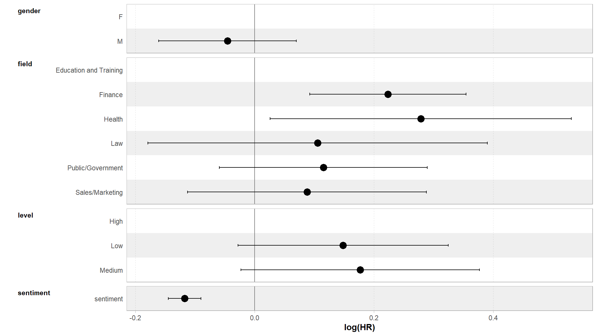
variable importance
feat_base <- names(job_retention)[c(1:4)]


fml_base = as.formula(paste0("Surv(time = month, event = left) ~ ",
                             paste(feat_base, collapse = " + ")))


cox_base_rms <- cph(fml_base, job_retention, x=TRUE, y=TRUE)
cox_base <- coxph(fml_base, job_retention)
cox_base_anova_rms <- anova(cox_base_rms)
plot(cox_base_anova_rms, sort = "ascending")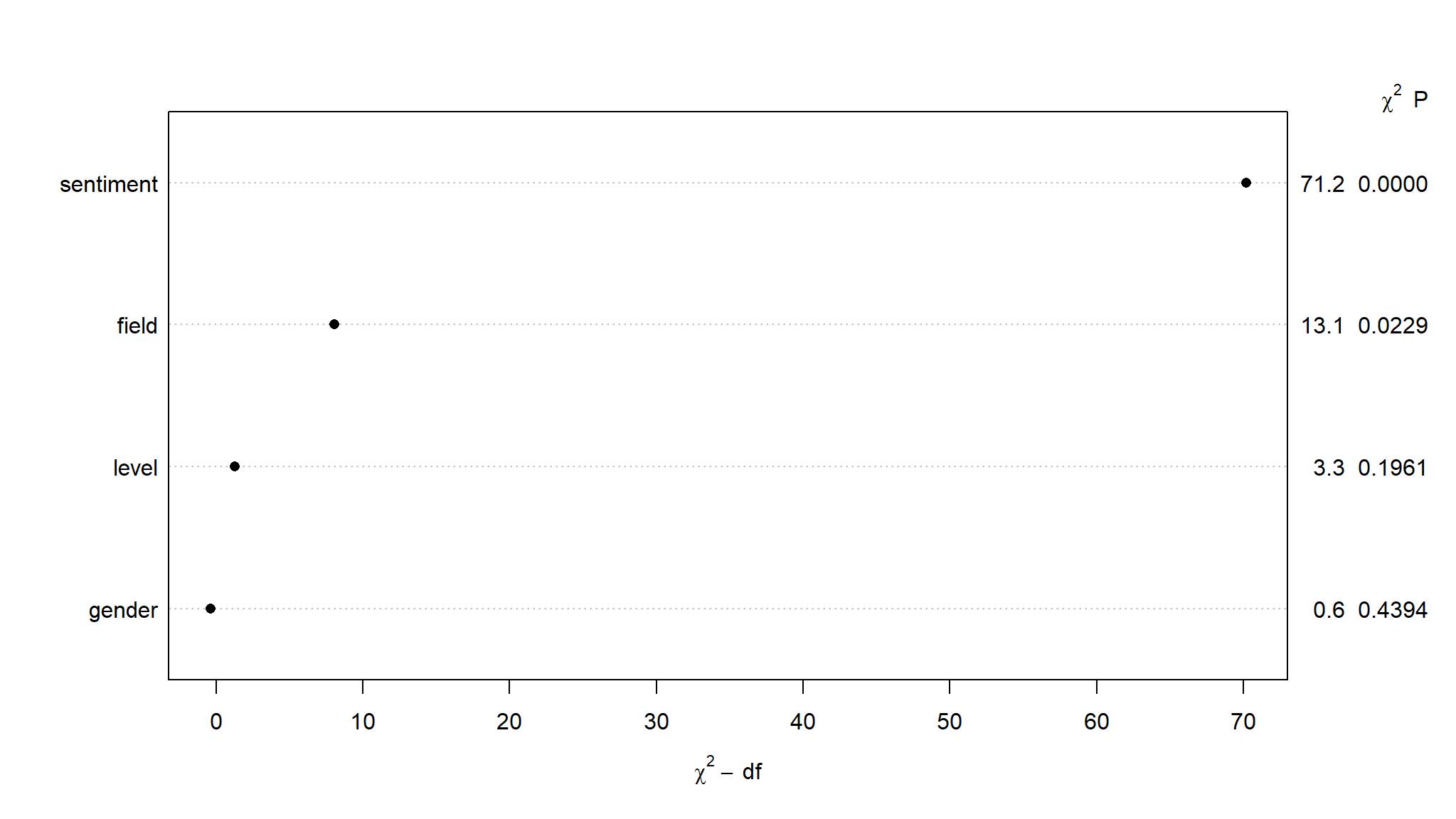
looks like sentiment has more impact in predicting job retention
feature_group <- function(x, feat) {
  for (i in 1:length(x)) {
    for (j in feat) {
      if (grepl(j, x[i])) {
        x[i] <- j
      }
    }
  }
  x
}

cox_base_coef <- summary(cox_base)
cox_base_coef <- tibble(Variable = row.names(cox_base_coef$coefficients),
                        group = feature_group(Variable, feat_base),
                        HR = cox_base_coef$coefficients[,2],
                        se = cox_base_coef$coefficients[,3]) %>%
  arrange(HR, group)

p1 <- ggplot(cox_base_coef, aes(x=Variable, y=HR, color=group)) +
  geom_hline(yintercept = 1) +
  geom_pointrange(aes(ymin=HR*exp(-1.96*se), ymax=HR*exp(1.96*se))) +
  scale_x_discrete(limits = cox_base_coef$Variable) +
  scale_color_manual(values = rev(paletteer_d("ggthemes::Tableau_10")[1:9])) +
  coord_flip() +
  labs(y = "Hazard Ratio [95% CI]", x = "", title = "Cox PH baseline, hazard ratios") +
  ggthemes::theme_tufte() +
  theme(legend.position = "none",
        plot.title = element_text(face = "bold", hjust = 0.5),
        axis.line = element_line(size = .2, color = "grey20"),
        axis.ticks.y = element_blank(),
        panel.grid.major.x = element_line(size=.2, color="grey90"),
        panel.grid.minor.x = element_line(size=.2, color="grey90"),
        panel.grid.major.y = element_line(size=.2, color="grey90", linetype="dotted"))

cox_coef <- summary(cox_base)
cox_coef <- tibble(Variable = row.names(cox_coef$coefficients),
                        group = feature_group(Variable, feat_base),
                        HR = cox_coef$coefficients[,2],
                        se = cox_coef$coefficients[,3]) %>%
  arrange(HR, group)

p2 <- ggplot(cox_coef, aes(x=Variable, y=HR, color=group)) +
  geom_hline(yintercept = 1) +
  geom_pointrange(aes(ymin=HR*exp(-1.96*se), ymax=HR*exp(1.96*se))) +
  scale_x_discrete(limits = cox_coef$Variable) +
  scale_color_manual(values = paletteer_d("ggthemes::Classic_20")[1:19]) +
  coord_flip() +
  labs(y = "Hazard Ratio [95% CI]", x = "", title = "Cox PH prev, hazard ratios") +
  ggthemes::theme_tufte() +
  theme(legend.position = "none",
        plot.title = element_text(face = "bold", hjust = 0.5),
        axis.line = element_line(size = .2, color = "grey20"),
        axis.ticks.y = element_blank(),
        panel.grid.major.x = element_line(size=.2, color="grey90"),
        panel.grid.minor.x = element_line(size=.2, color="grey90"),
        panel.grid.major.y = element_line(size=.2, color="grey90", linetype="dotted"))

ggarrange(p1,p2,nrow = 1,ncol = 2)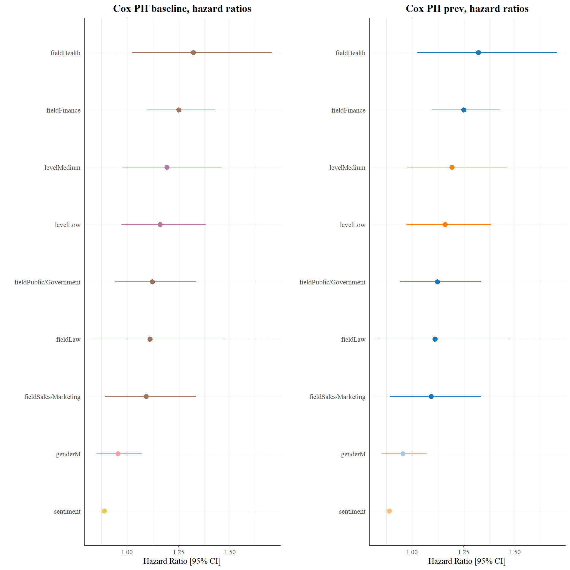
Checking the proportional hazard assumption
Note that we mentioned in the previous section a critical assumption for our Cox proportional hazard model to be valid, called the proportional hazard assumption. As always, it is important to check this assumption before finalizing any inferences or conclusions from your model.
The most popular test of this assumption uses a residual known as a Schoenfeld residual, which would be expected to be independent of time if the proportional hazard assumption holds. The cox.zph() function in the survival package runs a statistical test on the null hypothesis that the Schoenfeld residuals are independent of time. The test is conducted on every input variable and on the model as a whole, and a significant result would reject the proportional hazard assumption.
(ph_check <- survival::cox.zph(cox_model))
#>            chisq df    p
#> gender     0.726  1 0.39
#> field      6.656  5 0.25
#> level      2.135  2 0.34
#> sentiment  1.828  1 0.18
#> GLOBAL    11.156  9 0.27
In our case, we can confirm that the proportional hazard assumption is not rejected. The ggcoxzph() function in the survminer package takes the result of the cox.zph() check and allows a graphical check by plotting the residuals against time, as seen in Figure @ref(fig:schoenfeld).
survminer::ggcoxzph(ph_check,
                    font.main = 10,
                    font.x = 10,
                    font.y = 10)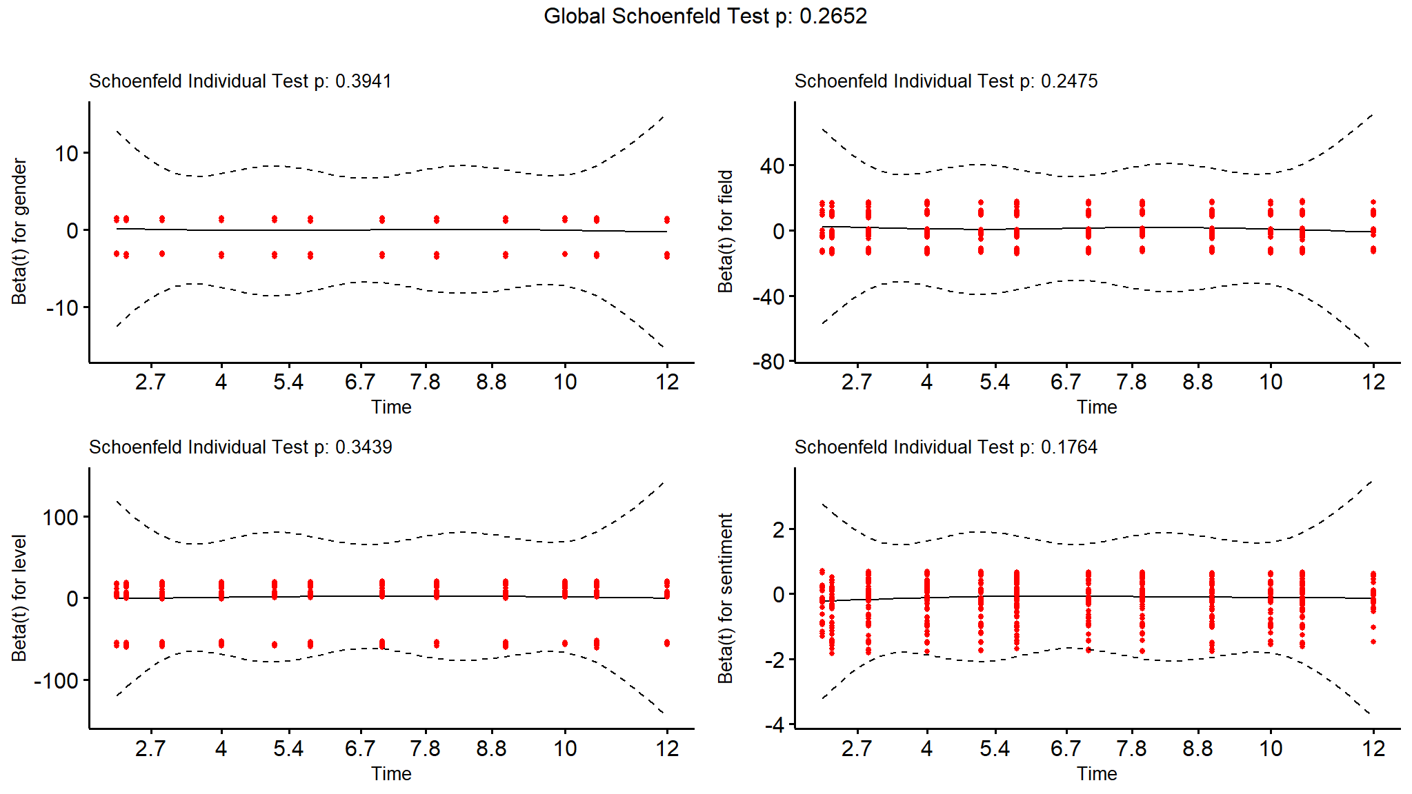
cox_modelAFT models
library(flexsurv)
par_fits <- tibble(
  dist_param = c("exp", "weibull", "gompertz","lognormal", "llogis"),
  dist_name = c("Exponential", "Weibull (AFT)", "Gompertz",
                "Lognormal", "Log-logistic")
) %>%
  mutate(
    fit = map(dist_param, ~flexsurvreg(Surv(month,left) ~ 1, data = job_retention, dist = .x)),
    fit_smry = map(fit, ~summary(.x, type = "hazard", ci = FALSE, tidy = TRUE)),
    AIC = map_dbl(fit, ~.x$AIC)
  )
par_fits %>%
dplyr::select(-c(dist_param, fit)) %>%
unnest(fit_smry) %>%
ggplot(aes(x = time, y = est, color = dist_name)) +
geom_line() +
theme_light() +
labs(title = "Parametric Distribution Fits to job retention data.")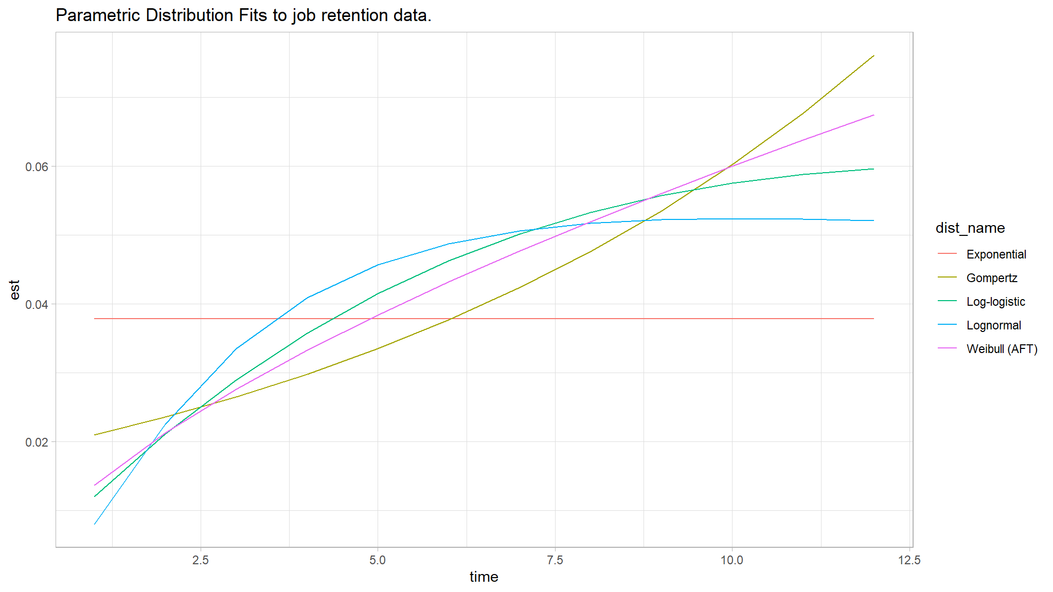
par_fits %>%
  arrange(AIC) %>%
  dplyr::select(dist_name, AIC)
#> # A tibble: 5 × 2
#>   dist_name        AIC
#>   <chr>          <dbl>
#> 1 Lognormal     11198.
#> 2 Log-logistic  11227.
#> 3 Weibull (AFT) 11248.
#> 4 Gompertz      11359.
#> 5 Exponential   11574.
we therefore attempt to use the lognormal model
rossi.phmodel<-survreg(Surv(event = left, time = month) ~ gender +
    field + level + sentiment,
  data = job_retention,dist="lognormal")
summary(rossi.phmodel)
#>
#> Call:
#> survreg(formula = Surv(event = left, time = month) ~ gender +
#>     field + level + sentiment, data = job_retention, dist = "lognormal")
#>                          Value Std. Error     z       p
#> (Intercept)             2.2474     0.1079 20.83 < 2e-16
#> genderM                 0.0178     0.0415  0.43 0.66886
#> fieldFinance           -0.1705     0.0466 -3.66 0.00025
#> fieldHealth            -0.2368     0.0916 -2.59 0.00971
#> fieldLaw               -0.0936     0.1019 -0.92 0.35821
#> fieldPublic/Government -0.1017     0.0617 -1.65 0.09940
#> fieldSales/Marketing   -0.1106     0.0702 -1.57 0.11530
#> levelLow               -0.0626     0.0607 -1.03 0.30233
#> levelMedium            -0.0931     0.0695 -1.34 0.18054
#> sentiment               0.0893     0.0104  8.58 < 2e-16
#> Log(scale)             -0.0271     0.0216 -1.25 0.21073
#>
#> Scale= 0.973
#>
#> Log Normal distribution
#> Loglik(model)= -5548.3   Loglik(intercept only)= -5597.2
#>  Chisq= 97.69 on 9 degrees of freedom, p= 4.6e-17
#> Number of Newton-Raphson Iterations: 3
#> n= 3770par(mfrow = c(1, 2), cex = 0.6)
lin.pred <- predict(rossi.phmodel, type = "lp")[job_retention$left == 1]
log.resid <- log(job_retention$month[job_retention$left == 1]) - lin.pred
plot(lin.pred, log.resid, main = "TA plot",
xlab = "log(fitted values)", ylab = "log(residuals)")
g<-qqPlot(log.resid, dist = "norm",
sd = rossi.phmodel$scale,
main = "Q-Q plot", xlab = "Theor. quantiles (normal)", ylab = "Emp. quantiles")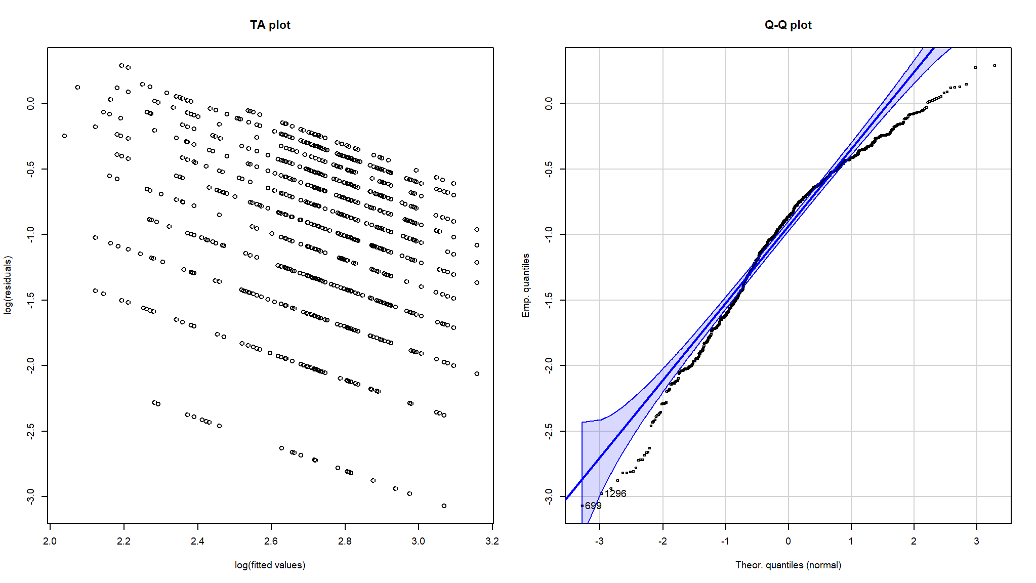
work in progress
Footnotes
The concordance measure returned is a measure of how well the model can predict in any given pair who will survive longer and is valuable in a number of medical research contexts.↩︎