Up and Running with SQL

Introduction to databases

We do realise that most of the softwares around are designed to solve a problem!. To better understand what databases are ,we need to first understand the problems that necessitated the advent of databases. The answer to this is quite obvious ! you have some data or large amounts of information that you need to store, this data could be about:

• Customers
• Products
• Employees etc

But why worry? , we could store the data in text files or even spreadsheets or if they are documents we can just organise them in folders…. is it! . Just having data is not a good enough reason to have a database , having data is not the problem but the problem is what comes next. Below are some of the problems that a database can solve

• size of the data
• ease of updating
• accuracy
• sensitivity
• redundancy
• importance

so what`s a database?

What is a database?

A structured storage space where the data is kept in many tables and organized so that the necessary information can be easily fetched, manipulated, and summarized.

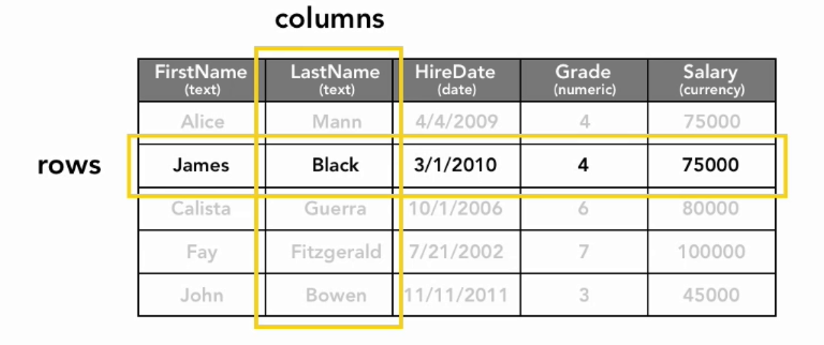
tables and fields

A table is an organized set of related data stored in a tabular form, i.e., in rows and columns. A field is another term for a column of a table and record is the other name for a row

Relational Data

Relational data are related by unique identifiers

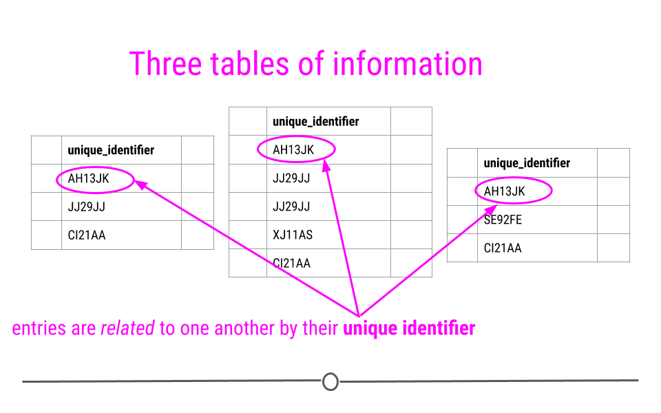
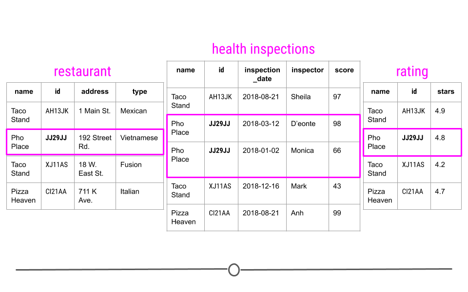
To better understand this, let’s consider a scenario were Bongani Has a business. say I have a number of different restaurants. In one table I might have information about these restaurants including, where they are located and what type of food they serve. I may then have a second table where information about health and safety inspections is stored. Each inspection is a different row and the date of the inspection, the inspector, and the safety rating are stored in this table. Finally, I might have a third table. This third table contains information pulled from an API, regarding the number of stars given to each restaurant, as rated by people online. Each table contains different bits of information; however, there is a common column id in each of the tables. This allows the information to be linked between the tables. The restaurant with the id “JJ29JJ” in the restaurant table would refer to the same restaurant with the id “JJ29JJ” in the health inspections table, and so on. The values in this id column are known as unique identifiers because they uniquely identify each restaurant. No two restaurants will have the same id, and the same restaurant will always have the same id, no matter what table you’re looking at. The fact that these tables have unique identifiers connecting each table to all the other tables makes this example what we call relational data.

Unique identifiers help link entries across tables

Why relational data?

Storing data in this way has a number of advantages; however, the three most important are:

1. Efficient Data Storage
2. Avoids Ambiguity
3. Privacy

DBMS

DDMS stands for Database Management System, a software package used to perform various operations on the data stored in a database, such as accessing, updating, wrangling, inserting, and removing data. There are various types of DBMS, such as relational, hierarchical, network, graph, or object-oriented. These types are based on the way the data is organized, structured, and stored in the system.

RDBMS

RDBMS stands for Relational Database Management System. It’s the most common type of DBMS used for working with data stored in multiple tables related to each other by means of shared keys. The SQL programming language is particularly designed to interact with RDBMS. Some examples of RDBMS are MySQL, PostgreSQL, Oracle, MariaDB, etc.

SQL constraints

constraints	Description
DEFAULT	provides a default value for a column
UNIQUE	allows only unique values
NOT NULL	allows only non-null values.
PRIMARY KEY	allows only unique and strictly non-null values (NOT NULL and UNIQUE).
FOREIGN KEY	provides shared keys between two and more tables

unique key

A column (or multiple columns) of a table to which the UNIQUE constraint was imposed to ensure unique values in that column, including a possible NULL value (the only one).

foreign key

A column (or multiple columns) of a table to which the FOREIGN KEY constraint was imposed to link this column to the primary key in another table (or several tables). The purpose of foreign keys is to keep connected various tables of a database.

SQL queries

A query is a piece of code written in SQL to access the data from a database or to modify the data. Correspondingly, there are two types of SQL queries: select and action queries. The first ones are used to retrieve the necessary data (this also includes limiting, grouping, ordering the data, extracting the data from multiple tables, etc.), while the second ones are used to create, add, delete, update, rename the data, etc.

SQL comments

A human-readable clarification on what a particular piece of code does. SQL code comments can be single-line (preceded by a double dash –) or span over multiple lines (as follows: /comment_text/). When the SQL engine runs, it ignores code comments. The purpose of adding SQL code comments is to make the code more comprehensive for those people who will read it in the future.

types of SQL commands (or SQL subsets)

Command	Explanation
Data Definition Language (DDL)	to define and modify the structure of a database.
Data Manipulation Language (DML)	to access, manipulate, and modify data in a database.
Data Control Language (DCL)	to control user access to the data in the database and give or, revoke privileges to a specific user or a group of users.
Transaction Control Language (TCL)	to control transactions in a database.
Data Query Language (DQL)	to perform queries on the data in a database to retrieve the necessary information from it.

creating a table

any computer system that deals with storing data needs to have the four fundamental functions that have the ability to:

• C-REATE
• R-EAD
• U-UPDATE
• D-ELETE

commonly pronounced as CRUD

we use the CREATE TABLE statement.

CREATE TABLE table_name (col_1 datatype,
                           col_2 datatype,
                           col_3 datatype);

for instance if run the following query !

CREATE TABLE my_table (age INTERGER,
                       sex TEXT);

we add the values to the table using INSERT INTO .... VALUES (....)

INSERT INTO my_table VALUES (34,'male');
INSERT INTO my_table VALUES (47,'female');
INSERT INTO my_table VALUES (32,'male');   

then call the database using SELECT

SELECT * FROM my_table;

#> # A tibble: 3 × 2
#>     age sex   
#>   <dbl> <chr> 
#> 1    34 male  
#> 2    47 female
#> 3    32 male

Querying a database

• we will use the Employee attrition database
• A query is a request for data from a database table (or combination of tables).
• Querying is an essential skill for a data scientist, since the data you need for your analyses will often live in databases.

SELECT statement

select all with *

• In SQL, you can select data from a table using a SELECT statement. For example, the following query selects the name column from the people table: SELECT name FROM people;
• you may want to select all columns from a table use * rather than typing all the columns

SELECT * FROM dat_new

#>    EmployeeNumber Attrition Age    BusinessTravel DailyRate
#> 1               1       Yes  41     Travel_Rarely      1102
#> 2               2        No  49 Travel_Frequently       279
#> 3               4       Yes  37     Travel_Rarely      1373
#> 4               5        No  33 Travel_Frequently      1392
#> 5               7        No  27     Travel_Rarely       591
#> 6               8        No  32 Travel_Frequently      1005
#> 7              10        No  59     Travel_Rarely      1324
#> 8              11        No  30     Travel_Rarely      1358
#> 9              12        No  38 Travel_Frequently       216
#> 10             13        No  36     Travel_Rarely      1299
#>                Department DistanceFromHome Education EducationField
#> 1                   Sales                1         2  Life Sciences
#> 2  Research & Development                8         1  Life Sciences
#> 3  Research & Development                2         2          Other
#> 4  Research & Development                3         4  Life Sciences
#> 5  Research & Development                2         1        Medical
#> 6  Research & Development                2         2  Life Sciences
#> 7  Research & Development                3         3        Medical
#> 8  Research & Development               24         1  Life Sciences
#> 9  Research & Development               23         3  Life Sciences
#> 10 Research & Development               27         3        Medical
#>    EmployeeCount EnvironmentSatisfaction Gender HourlyRate JobInvolvement
#> 1              1                       2 Female         94              3
#> 2              1                       3   Male         61              2
#> 3              1                       4   Male         92              2
#> 4              1                       4 Female         56              3
#> 5              1                       1   Male         40              3
#> 6              1                       4   Male         79              3
#> 7              1                       3 Female         81              4
#> 8              1                       4   Male         67              3
#> 9              1                       4   Male         44              2
#> 10             1                       3   Male         94              3
#>    JobLevel                   JobRole JobSatisfaction MaritalStatus
#> 1         2           Sales Executive               4        Single
#> 2         2        Research Scientist               2       Married
#> 3         1     Laboratory Technician               3        Single
#> 4         1        Research Scientist               3       Married
#> 5         1     Laboratory Technician               2       Married
#> 6         1     Laboratory Technician               4        Single
#> 7         1     Laboratory Technician               1       Married
#> 8         1     Laboratory Technician               3      Divorced
#> 9         3    Manufacturing Director               3        Single
#> 10        2 Healthcare Representative               3       Married
#>    MonthlyIncome MonthlyRate NumCompaniesWorked Over18 OverTime
#> 1           5993       19479                  8      Y      Yes
#> 2           5130       24907                  1      Y       No
#> 3           2090        2396                  6      Y      Yes
#> 4           2909       23159                  1      Y      Yes
#> 5           3468       16632                  9      Y       No
#> 6           3068       11864                  0      Y       No
#> 7           2670        9964                  4      Y      Yes
#> 8           2693       13335                  1      Y       No
#> 9           9526        8787                  0      Y       No
#> 10          5237       16577                  6      Y       No
#>    PercentSalaryHike PerformanceRating RelationshipSatisfaction StandardHours
#> 1                 11                 3                        1            80
#> 2                 23                 4                        4            80
#> 3                 15                 3                        2            80
#> 4                 11                 3                        3            80
#> 5                 12                 3                        4            80
#> 6                 13                 3                        3            80
#> 7                 20                 4                        1            80
#> 8                 22                 4                        2            80
#> 9                 21                 4                        2            80
#> 10                13                 3                        2            80
#>    StockOptionLevel TotalWorkingYears TrainingTimesLastYear WorkLifeBalance
#> 1                 0                 8                     0               1
#> 2                 1                10                     3               3
#> 3                 0                 7                     3               3
#> 4                 0                 8                     3               3
#> 5                 1                 6                     3               3
#> 6                 0                 8                     2               2
#> 7                 3                12                     3               2
#> 8                 1                 1                     2               3
#> 9                 0                10                     2               3
#> 10                2                17                     3               2
#>    YearsAtCompany YearsInCurrentRole YearsSinceLastPromotion
#> 1               6                  4                       0
#> 2              10                  7                       1
#> 3               0                  0                       0
#> 4               8                  7                       3
#> 5               2                  2                       2
#> 6               7                  7                       3
#> 7               1                  0                       0
#> 8               1                  0                       0
#> 9               9                  7                       1
#> 10              7                  7                       7
#>    YearsWithCurrManager
#> 1                     5
#> 2                     7
#> 3                     0
#> 4                     0
#> 5                     2
#> 6                     6
#> 7                     0
#> 8                     0
#> 9                     8
#> 10                    7

selecting a subset

• you can achieve this by defining the columns to be selected e.g

SELECT col_1,col_2,col_3 
FROM my_table;

using the database we get

SELECT Attrition,Department,Education 
FROM dat_new;

#>    Attrition             Department Education
#> 1        Yes                  Sales         2
#> 2         No Research & Development         1
#> 3        Yes Research & Development         2
#> 4         No Research & Development         4
#> 5         No Research & Development         1
#> 6         No Research & Development         2
#> 7         No Research & Development         3
#> 8         No Research & Development         1
#> 9         No Research & Development         3
#> 10        No Research & Development         3

select distinct items in SQL

• Often your results will include many duplicate values. If you want to select all the unique values from a column, you can use the DISTINCT keyword. for instance if you have the following database table:

#> # A tibble: 5 × 3
#>   Name      age sex   
#>   <chr>   <dbl> <chr> 
#> 1 Bongani    34 male  
#> 2 Eliza      47 female
#> 3 Bongani    34 male  
#> 4 Peter      27 male  
#> 5 Fadzie     19 female

• we can see that Bongani has been recorded twice in the dataset

SELECT DISTINCT name,age,sex 
FROM database_table

#>      Name age    sex
#> 1 Bongani  34   male
#> 2   Eliza  47 female
#> 3   Peter  27   male
#> 4  Fadzie  19 female

filtering using WHERE in SQL

• WHERE is a filtering clause

• In SQL, the WHERE keyword allows you to filter based on both text and numeric values in a table. There are a few different comparison operators you can use:

• = equal

• <> not equal

• < less than

• > greater than

• <= less than or equal to

• >= greater than or equal to

• You can build up your WHERE queries by combining multiple conditions with the AND keyword.

SELECT DISTINCT name,age,sex
FROM df
WHERE sex='male';

#>      Name age  sex
#> 1 Bongani  34 male
#> 2   Peter  27 male

COUNT and AS alias in SQL

• The COUNT statement lets you count then returning the number of rows in one or more columns.
• we use AS to rename default name
• COUNT(*) tells you how many rows are in a table

SELECT COUNT(*) AS pple_count
FROM database_table;

#>   pple_count
#> 1          5

• the above query calculates the number of rows in the data and finds 5 rows

we can use COUNT(DISTINCT column) to get the number of unique rows

SELECT COUNT(DISTINCT name) AS unique_count
FROM database_table;

#>   unique_count
#> 1            4

the query above will calculate rows with distinct names and finds them to be 4

We can use COUNT with WHERE

• We can do this to get the number of terms after filtering
• how many people are male?

SELECT COUNT(*) AS num_male
FROM database_table
WHERE sex='male';

#>   num_male
#> 1        3

Manipulating and Aggregating

Create a database for the exercises

con<-dbConnect(RSQLite::SQLite(), ":memory:")
copy_to(con,data1)
copy_to(con,data2)

filtering using WHERE in SQL

the following points were outlined previously

• WHERE is a filtering clause

• In SQL, the WHERE keyword allows you to filter based on both text and numeric values in a table. There are a few different comparison operators you can use:

• = equal

• <> not equal

• < less than

• > greater than

• <= less than or equal to

• >= greater than or equal to

• You can build up your WHERE queries by combining multiple conditions with the AND keyword.

SELECT * 
FROM data2 
WHERE category='Potato'

1 records

recipe	calories	sugar	protein	category
624	236.62	0.81	9.07	Potato

filtering using IN and WHERE in SQL

SELECT * 
FROM data2 
WHERE category IN ('Chicken','Chicken Breast')

5 records

recipe	calories	sugar	protein	category
609	NA	NA	NA	Chicken Breast
671	481.88	1.34	51.90	Chicken
683	147.24	0.94	54.00	Chicken
419	1830.28	1.83	44.74	Chicken Breast
117	NA	NA	NA	Chicken Breast

COUNT and AS alias in SQL

• The COUNT statement lets you count then returning the number of rows in one or more columns.
• we use AS to rename default name
• COUNT(*) tells you how many rows are in a table

SELECT COUNT(*) AS n 
FROM data2

1 records

n
25

count filters in SQL

SELECT COUNT(category) AS n_potato
FROM data2 
WHERE category IN ('Chicken Breast','Chicken')

1 records

n_potato
5

Updating a database using dbExecute

• categories before

#>        category n percent
#>       Beverages 1    0.04
#>       Breakfast 4    0.16
#>         Chicken 2    0.08
#>  Chicken Breast 3    0.12
#>         Dessert 3    0.12
#>            Meat 4    0.16
#>   One Dish Meal 3    0.12
#>            Pork 1    0.04
#>          Potato 1    0.04
#>       Vegetable 3    0.12

Updating a database

• we need to change a category called Breakfast to Breakfast meal
• we shall use REPLACE

UPDATE data2 
SET category= REPLACE(category,'Breakfast','Breakfast meal')
WHERE category='Breakfast'

Querying to check results

SELECT category, COUNT(category) as n_per_category
FROM data2
GROUP BY category

Displaying records 1 - 10

category	n_per_category
Beverages	1
Breakfast meal	4
Chicken	2
Chicken Breast	3
Dessert	3
Meat	4
One Dish Meal	3
Pork	1
Potato	1
Vegetable	3

• we see that Breakfast has updated to Breakfast meal

Missing data in SQL

• in SQL, NULL represents a missing or unknown value. You can check for NULL values using the expression IS NULL
• Use IS NULL AND IS NOT NULL

filtering missing data

SELECT * 
FROM data2 
WHERE Protein IS NULL

3 records

recipe	calories	sugar	protein	category
912	NA	NA	NA	Dessert
609	NA	NA	NA	Chicken Breast
117	NA	NA	NA	Chicken Breast

filtering nonmissing data

SELECT * 
FROM data2 
WHERE Protein IS NOT NULL

Displaying records 1 - 10

recipe	calories	sugar	protein	category
624	236.62	0.81	9.07	Potato
102	198.98	0.39	39.12	Vegetable
427	187.41	86.97	4.49	Dessert
324	49.50	4.69	53.33	Breakfast meal
380	75.89	8.18	17.64	Meat
671	481.88	1.34	51.90	Chicken
683	147.24	0.94	54.00	Chicken
208	20.98	9.80	0.82	Beverages
633	105.95	0.07	7.55	Vegetable
859	388.44	4.62	13.93	Pork

How many categories do we have

select distinct items in SQL

• Often your results will include many duplicate values. If you want to select all the unique values from a column, you can use the DISTINCT keyword.

SELECT COUNT(DISTINCT category) AS unique_categories 
FROM data2

1 records

unique_categories
10

Advanced filters

filtering in SQL

SELECT * 
FROM data2 WHERE sugar > 1 AND sugar < 5 
AND category='Breakfast meal'

3 records

recipe	calories	sugar	protein	category
324	49.5	4.69	53.33	Breakfast meal
598	212.4	2.25	23.78	Breakfast meal
526	93.5	2.57	23.68	Breakfast meal

• also achieved by using BETWEEN and AND

SELECT * 
FROM data2 
WHERE sugar BETWEEN 1 AND 5 
AND category='Breakfast meal'

3 records

recipe	calories	sugar	protein	category
324	49.5	4.69	53.33	Breakfast meal
598	212.4	2.25	23.78	Breakfast meal
526	93.5	2.57	23.68	Breakfast meal

filtering text data in SQL

• use LIKE
• the LIKE operator can be used in a WHERE clause to search for a pattern in a column.
• To accomplish this, you use something called a wildcard as a placeholder for some other values. There are two wildcards you can use with LIKE:

The % wildcard will match zero, one, or many characters in text

The _ wildcard will match a single character

SELECT * 
FROM data2 
WHERE category LIKE 'Chicken%'

5 records

recipe	calories	sugar	protein	category
609	NA	NA	NA	Chicken Breast
671	481.88	1.34	51.90	Chicken
683	147.24	0.94	54.00	Chicken
419	1830.28	1.83	44.74	Chicken Breast
117	NA	NA	NA	Chicken Breast

Aggregate functions in SQL

SELECT AVG(sugar) AS avg_sugar,
       MAX(sugar) AS max_sugar,
       MIN(sugar) AS min_sugar,
       VARIANCE(sugar) AS variance,
       STDEV(sugar) AS stnd_deviation
FROM data2;

1 records

avg_sugar	max_sugar	min_sugar	variance	stnd_deviation
11.24864	86.97	0.07	426.5449	20.65296

Grouping and aggregating in SQL

SELECT category,AVG(sugar) AS avg_sugar,
                       MAX(sugar) AS max_sugar,
                       MIN(sugar) AS min_sugar
FROM data2
GROUP BY category;

Displaying records 1 - 10

category	avg_sugar	max_sugar	min_sugar
Beverages	9.8000000	9.80	9.80
Breakfast meal	5.1600000	11.13	2.25
Chicken	1.1400000	1.34	0.94
Chicken Breast	1.8300000	1.83	1.83
Dessert	69.5700000	86.97	52.17
Meat	13.5525000	30.06	5.21
One Dish Meal	3.9066667	6.09	1.46
Pork	4.6200000	4.62	4.62
Potato	0.8100000	0.81	0.81
Vegetable	0.8066667	1.96	0.07

we can order the data by a certain column using ORDER BY clause

SELECT category,AVG(sugar) AS avg_sugar,
                       MAX(sugar) AS max_sugar,
                       MIN(sugar) AS min_sugar
FROM data2
GROUP BY category
ORDER BY avg_sugar;

Displaying records 1 - 10

category	avg_sugar	max_sugar	min_sugar
Vegetable	0.8066667	1.96	0.07
Potato	0.8100000	0.81	0.81
Chicken	1.1400000	1.34	0.94
Chicken Breast	1.8300000	1.83	1.83
One Dish Meal	3.9066667	6.09	1.46
Pork	4.6200000	4.62	4.62
Breakfast meal	5.1600000	11.13	2.25
Beverages	9.8000000	9.80	9.80
Meat	13.5525000	30.06	5.21
Dessert	69.5700000	86.97	52.17

the above output shows results arranged in ascending order of avg_sugar , if we needed to begin with the largest descending we could useORDER BY...DESC

SELECT category,AVG(sugar) AS avg_sugar,
                       MAX(sugar) AS max_sugar,
                       MIN(sugar) AS min_sugar
FROM data2
GROUP BY category
ORDER BY avg_sugar DESC;

Displaying records 1 - 10

category	avg_sugar	max_sugar	min_sugar
Dessert	69.5700000	86.97	52.17
Meat	13.5525000	30.06	5.21
Beverages	9.8000000	9.80	9.80
Breakfast meal	5.1600000	11.13	2.25
Pork	4.6200000	4.62	4.62
One Dish Meal	3.9066667	6.09	1.46
Chicken Breast	1.8300000	1.83	1.83
Chicken	1.1400000	1.34	0.94
Potato	0.8100000	0.81	0.81
Vegetable	0.8066667	1.96	0.07

Using UPPER()

Sometimes you may want to change a column to all upper cases

SELECT recipe,category , UPPER(category) AS upper_cat
FROM data2;

Displaying records 1 - 10

recipe	category	upper_cat
624	Potato	POTATO
102	Vegetable	VEGETABLE
427	Dessert	DESSERT
324	Breakfast meal	BREAKFAST MEAL
912	Dessert	DESSERT
380	Meat	MEAT
609	Chicken Breast	CHICKEN BREAST
671	Chicken	CHICKEN
683	Chicken	CHICKEN
208	Beverages	BEVERAGES

Basic arithmetic

• In addition to using aggregate functions, you can perform basic arithmetic with symbols like +, -, *, and /.
• lets create weird variables here

SELECT category,(sugar-protein) AS diff_sugar_protein 
FROM data2;

Displaying records 1 - 10

category	diff_sugar_protein
Potato	-8.26
Vegetable	-38.73
Dessert	82.48
Breakfast meal	-48.64
Dessert	NA
Meat	-9.46
Chicken Breast	NA
Chicken	-50.56
Chicken	-53.06
Beverages	8.98

CASE statements

this contains a WHEN,THEN and ELSE statement ,finished with END

Take the stair CASE

• using CASE WHEN to categorise or group data as follows
• SELECT….
• CASE WHEN condition THEN category
• WHEN condition THEN category
• …………………………………..
• ELSE some_category
• END AS variable name

SELECT recipe , sugar,
   CASE WHEN sugar BETWEEN 0 AND 50 THEN '0-50'
        WHEN sugar BETWEEN 51 AND 100 THEN '51-100'
        WHEN sugar BETWEEN 101 AND 200 THEN '101-200'
        WHEN sugar IS NULL THEN 'missing'
        ELSE '>200'
        END AS sugar_category
FROM data2;

Displaying records 1 - 10

recipe	sugar	sugar_category
624	0.81	0-50
102	0.39	0-50
427	86.97	51-100
324	4.69	0-50
912	NA	missing
380	8.18	0-50
609	NA	missing
671	1.34	0-50
683	0.94	0-50
208	9.80	0-50

we can letter perform aggregations on the new column for instance get the count per each category

SELECT COUNT(*) AS count_per_category,
   CASE WHEN sugar BETWEEN 0 AND 50 THEN '0-50'
        WHEN sugar BETWEEN 51 AND 100 THEN '51-100'
        WHEN sugar BETWEEN 101 AND 200 THEN '101-200'
        WHEN sugar IS NULL THEN 'missing'
        ELSE '>200'
        END AS sugar_category
FROM data2
GROUP BY sugar_category;

3 records

count_per_category	sugar_category
20	0-50
2	51-100
3	missing

SQL subqueries

A subquery is a query nested in another query and is useful for intermediate transformations

SELECT column
FROM (SELECT column 
      FROM table) AS subquery;

subqueries can be found anywhere within SELECT,FROM,WHERE,GROUP BY

use cases

• comparing groups to summarised values
• Reshaping Data
• Combining data that cannot be joined

for instance

• use data1 and data2 databases for this task
• the following is just an example and calories in data2 and data1 are the same so the result is the same

SELECT recipe,calories
FROM data2 
WHERE calories > 
      (SELECT AVG(calories) FROM data1);

9 records

recipe	calories
671	481.88
859	388.44
171	431.28
282	409.99
91	388.37
868	307.36
885	504.09
419	1830.28
639	321.95

Summarize group statistics using subqueries

Sometimes you want to understand how a value varies across groups. For example, how does the maximum value per group vary across groups?

To find out, first summarize by group, and then compute summary statistics of the group results. One way to do this is to compute group values in a subquery, and then summarize the results of the subquery.

what is the standard deviation across meal cateries in the maximum amount of sugar? What about the mean, min, and max of the maximums as well?

Start by writing a subquery to compute the max() per categoy; alias the subquery result as sugar_max. Then compute the standard deviation of sugar_max with stddev(). Compute the min(), max(), and avg() of sugar_max too.

SELECT AVG(sugar_max) AS avg_sugar,
       MAX(sugar_max) AS max_sugar,
       MIN(sugar_max) AS min_sugar,
       VARIANCE(sugar_max) AS variance,
       STDEV(sugar_max) AS stnd_deviation
FROM (SELECT MAX(sugar) AS sugar_max
      FROM data2
         -- Compute max by...
      GROUP BY category) AS max_results

1 records

avg_sugar	max_sugar	min_sugar	variance	stnd_deviation
15.461	86.97	0.81	707.2168	26.59355

SQL JOINS

setting up the data

• to aid with illustrations , I have created some fake datasets to assist in explaining and these are join_df1.csv and join_df2.csv datasets
• read in CSV files and store them as databases in R

# read in example csv files (join_df1 and join_df2)
join_df1 <- read.csv("join_df1.csv") |> 
  dplyr::rename(A=bongi)
join_df2 <- read.csv("join_df2.csv")|> 
  dplyr::rename(A=bongi)

join<-dbConnect(RSQLite::SQLite(), ":memory:")
copy_to(join,join_df1)
copy_to(join,join_df2)

join_df1

SELECT * FROM join_df1

8 records

A	B	C
red	2	3
orange	4	6
yellow	8	9
green	0	0
indigo	3	3
blue	1	1
purple	5	5
white	8	2

this data has 8 rows and 3 columns

join_df2

SELECT * FROM join_df2

7 records

A	D
red	3
orange	5
yellow	7
green	1
indigo	3
blue	6
pink	9

this has 7 rows and 2 columns

• note that we will use the column A as our unique identifier

Querying A join

generally the following step show how a join is done in SQL

• SELECT t1.comon_column1,t1.common_column2,…
• FROM table1 AS t1
• <type> JOIN table2 AS t2
• ON t1.common_unique_column = t2.common_unique_column;

Inner Join

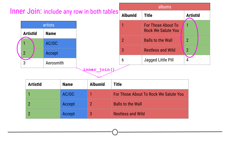
When talking about inner joins, we are only going to keep an observation if it is found in all of the tables we’re combining. Here, we’re combining the tables based on the ArtistId column. In our dummy example, there are only two artists that are found in both tables. These are highlighted in green and will be the rows used to join the two tables. Then, once the inner join happens, only these artists’ data will be included after the inner join.

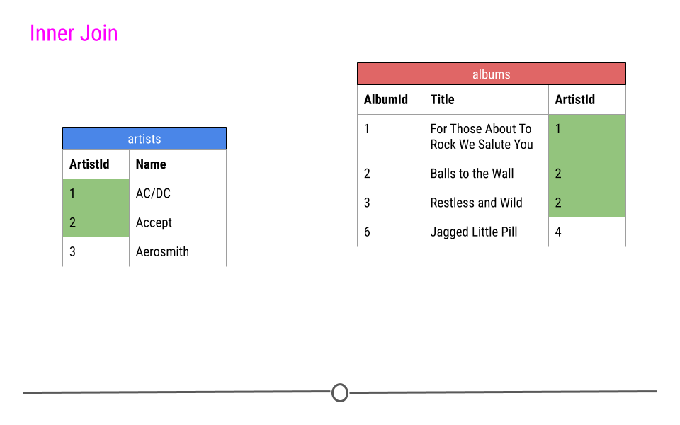
when doing an inner join, data from any observation found in all the tables being joined are included in the output. Here, ArtistIds “1” and “2” are in both the artists and albums tables. Thus, those will be the only ArtistIds in the output from the inner join.

And, since it’s a mutating join, our new table will have information from both tables! We now have ArtistId, Name, AlbumId, and Title in a single table! We’ve joined the two tables, based on the column ArtistId!

See this in ACTION

SELECT * 
FROM join_df1
INNER JOIN join_df2
USING(A)

6 records

A	B	C	D
red	2	3	3
orange	4	6	5
yellow	8	9	7
green	0	0	1
indigo	3	3	3
blue	1	1	6

we note from the above that only the colours that are common to both tables are returned. however instead of using USING we can use ON table1.columnname=table2.columnname where columnname is the column that tables to be matched by and in our example this is column A . when using this method it is important to give each table an ALIAS which is a shorthand for our tables

SELECT * 
FROM join_df1 AS j1
INNER JOIN join_df2 AS j2
ON j1.A=j2.A;            

6 records

A	B	C	A	D
red	2	3	red	3
orange	4	6	orange	5
yellow	8	9	yellow	7
green	0	0	green	1
indigo	3	3	indigo	3
blue	1	1	blue	6

looking at the table above ,we note that column A has been repeated twice , thus we need to only SELECT the column A From only one of our tables hence we specify the repeated columns in the SELECT statement using the table.columnname method . So in the example above SELECT j1.A,B,C,D specifies that we want we want column A to come from table j1 (j1.A)

SELECT j1.A,B,C,D 
FROM join_df1 AS j1
INNER JOIN join_df2 AS j2
ON j1.A=j2.A;

6 records

A	B	C	D
red	2	3	3
orange	4	6	5
yellow	8	9	7
green	0	0	1
indigo	3	3	3
blue	1	1	6

great :)! , generally we can apply the same scenario to all kinds of joins

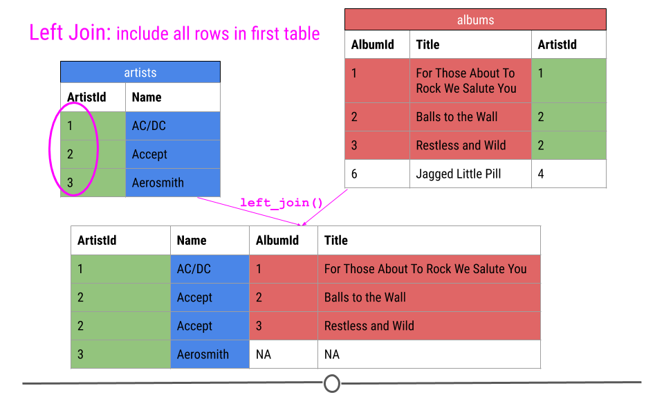
left join in SQL

For a left join, all rows in the first table specified will be included in the output. Any row in the second table that is not in the first table will not be included.

In our toy example this means that ArtistIDs 1, 2, and 3 will be included in the output; however, ArtistID 4 will not.

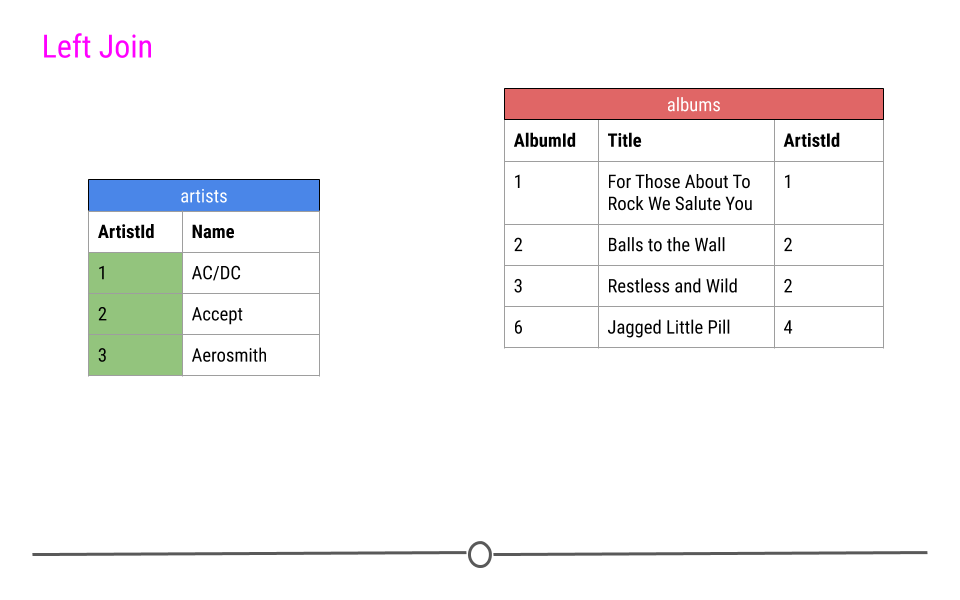
Thus, our output will again include all the columns from both tables combined into a single table; however, for ArtistId 3, there will be NAs for AlbumId and Title. NAs will be filled in for any observations in the first table specified that are missing in the second table.

Let us see it in ACTION

SELECT j1.A,B,C,D 
FROM join_df1 AS j1
LEFT JOIN join_df2 AS j2
ON j1.A=j2.A;

8 records

A	B	C	D
red	2	3	3
orange	4	6	5
yellow	8	9	7
green	0	0	1
indigo	3	3	3
blue	1	1	6
purple	5	5	NA
white	8	2	NA

great , we notice the NA values found in the last column

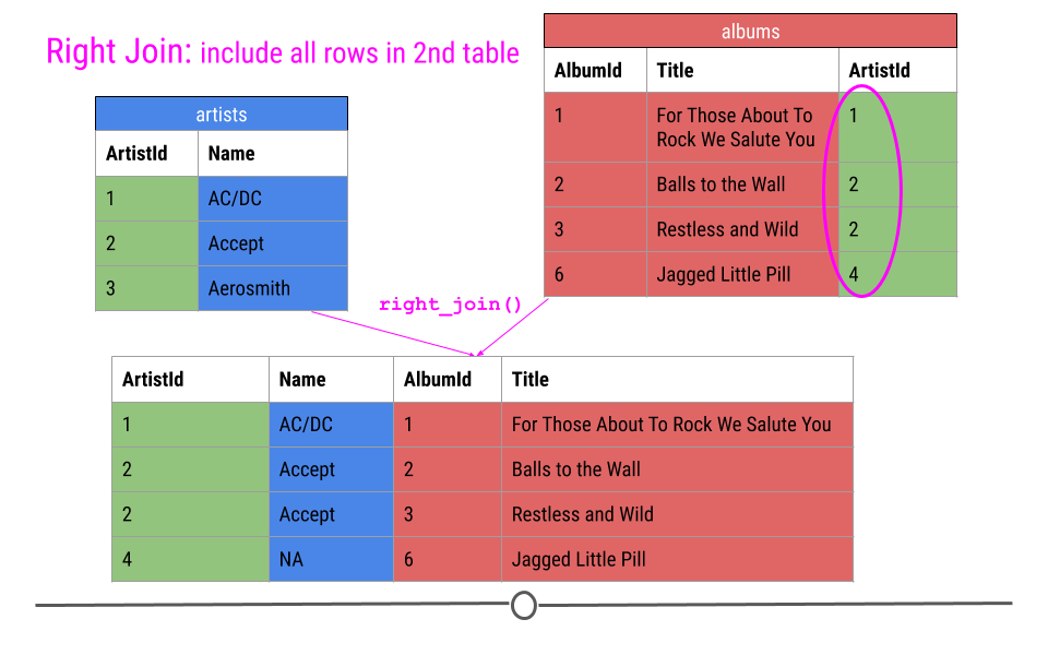
RIGHT JOIN IN SQL

Right Join is similar to what we just discussed; however, in the output from a right join, all rows in the final table specified are included in the output. NAs will be included for any observations found in the last specified table but not in the other tables.

In our toy example, that means, information about ArtistIDs 1, 2, and 4 will be included.

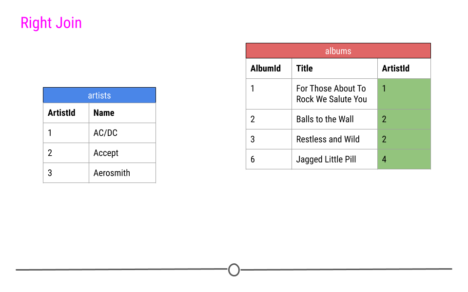
Again, in our toy example, we see that right join combines the information across tables; however, in this case, ArtistId 4 is included, but Name is an NA, as this information was not in the artists table for this artist.

Let us see a RIGHT JOIN in action

SELECT j1.A,B,C,D 
FROM join_df1 AS j1
RIGHT JOIN join_df2 AS j2
ON j1.A=j2.A;

7 records

A	B	C	D
red	2	3	3
orange	4	6	5
yellow	8	9	7
green	0	0	1
indigo	3	3	3
blue	1	1	6
NA	NA	NA	9

great , notice now where the NA is displayed

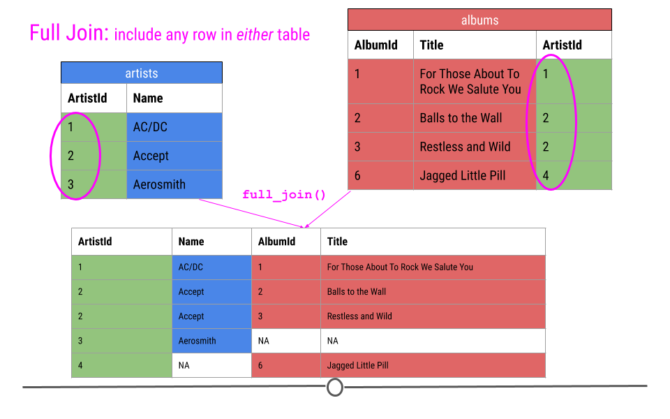
full join in SQL

Finally, a full join will take every observation from every table and include it in the output.

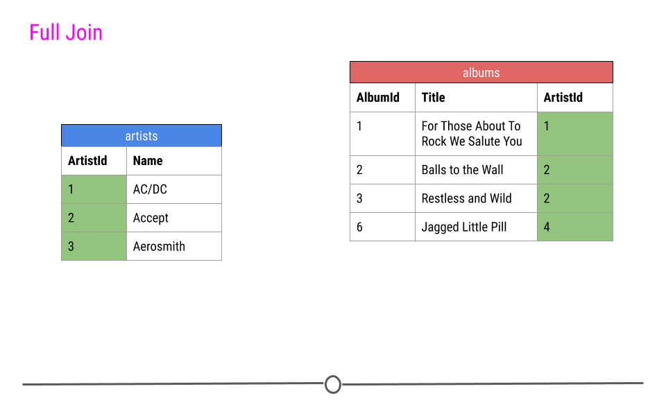
Thus, in our toy example, this join produces five rows, including all the observations from either table. NAs are filled in when data are missing for an observation.

let us see a FULL JOIN in ACTION

SELECT j1.A,B,C,D 
FROM join_df1 AS j1
FULL JOIN join_df2 AS j2
ON j1.A=j2.A;

9 records

A	B	C	D
red	2	3	3
orange	4	6	5
yellow	8	9	7
green	0	0	1
indigo	3	3	3
blue	1	1	6
purple	5	5	NA
white	8	2	NA
NA	NA	NA	9

Window functions

• A window function performs an aggregate-like operation on a set of query rows.

However, whereas an aggregate operation groups query rows into a single result row, a window function produces a result for each query row:

Anatomy of a window function

• FUNCTION_NAME() OVER()
• ORDER BY
• PARTITION BY
• ROWS/RANGE PRECEDING/FOLLOWING/UNBOUNDED

Creating a fake dataset in R

library(tidyverse)

sales<-tribble(~ year , ~country , ~product    , ~profit ,~Own ,~Time,
                 2000 , "Finland", "Computer"  ,   1500  ,"Y"  ,"D",
                 2000 , "Finland" ,"Phone"      ,   100   ,"Y"  ,"D",
                 2001 , "Finland" ,"Phone"      ,     10  ,"N"  ,"D",
                 2000 , "India"   ,"Calculator" ,     75  ,"Y"  ,"E",
                 2000 , "India"   ,"Calculator" ,     75  ,"N"  ,"E",
                 2000 , "India"   ,"Computer"   ,   1200  ,"N"  ,"E",
                 2000 , "USA"     , "Calculator",     75  ,"Y"  ,"E",
                 2000 , "USA"     , "Computer"  ,   1500  ,"N"  ,"E",
                 2001 , "USA"     ,"Calculator" ,     50  ,"Y"  ,"E",
                 2001 , "USA"     ,"Computer"   ,   1500  ,"Y"  ,"E",
                 2001 , "USA"     ,"Computer"   ,   1200  ,"Y"  ,"D",
                 2001 , "USA"     , "TV"        ,    150  ,"Y"  ,"D",
                 2001 , "USA"     , "TV"        ,    100  ,"Y"  ,"D")
sales
#> # A tibble: 13 × 6
#>     year country product    profit Own   Time 
#>    <dbl> <chr>   <chr>       <dbl> <chr> <chr>
#>  1  2000 Finland Computer     1500 Y     D    
#>  2  2000 Finland Phone         100 Y     D    
#>  3  2001 Finland Phone          10 N     D    
#>  4  2000 India   Calculator     75 Y     E    
#>  5  2000 India   Calculator     75 N     E    
#>  6  2000 India   Computer     1200 N     E    
#>  7  2000 USA     Calculator     75 Y     E    
#>  8  2000 USA     Computer     1500 N     E    
#>  9  2001 USA     Calculator     50 Y     E    
#> 10  2001 USA     Computer     1500 Y     E    
#> 11  2001 USA     Computer     1200 Y     D    
#> 12  2001 USA     TV            150 Y     D    
#> 13  2001 USA     TV            100 Y     D

Load in the necessary packages

library(odbc)
library(DBI)
library(RSQLite)

Set up a database using the datafile

wind<-dbConnect(RSQLite::SQLite(), ":memory:")
copy_to(wind,sales)

Lets get started

• The row for which function evaluation occurs is called the current row.
• The query rows related to the current row over which function evaluation occurs comprise the window for the current row.

ROW_NUMBER() OVER()

• use it if maybe you have duplicates or intend to create rowids for your data

SELECT ROW_NUMBER() OVER () AS row_id , year, country, product, profit
FROM sales;

Displaying records 1 - 10

row_id	year	country	product	profit
1	2000	Finland	Computer	1500
2	2000	Finland	Phone	100
3	2001	Finland	Phone	10
4	2000	India	Calculator	75
5	2000	India	Calculator	75
6	2000	India	Computer	1200
7	2000	USA	Calculator	75
8	2000	USA	Computer	1500
9	2001	USA	Calculator	50
10	2001	USA	Computer	1500

PARTITION BY

• This splits the table into partitions based on a column’s unique values and results aren’t rolled into one column

therefore ROW_NUMBER() With PARTITION BY produces the row number of each row within its partition. In this case, rows are numbered per country. By default, partition rows are unordered and row numbering is nondeterministic.

SELECT ROW_NUMBER() OVER(PARTITION BY country) AS row_num1,
       year, country, product, profit
FROM sales;

Displaying records 1 - 10

row_num1	year	country	product	profit
1	2000	Finland	Computer	1500
2	2000	Finland	Phone	100
3	2001	Finland	Phone	10
1	2000	India	Calculator	75
2	2000	India	Calculator	75
3	2000	India	Computer	1200
1	2000	USA	Calculator	75
2	2000	USA	Computer	1500
3	2001	USA	Calculator	50
4	2001	USA	Computer	1500

its also possible to use ROW_NUMBER() With ORDER BY to determine ranks

SELECT ROW_NUMBER() OVER(ORDER BY profit DESC) AS row_num1,
       year, country, product, profit
FROM sales;

Displaying records 1 - 10

row_num1	year	country	product	profit
1	2000	Finland	Computer	1500
2	2000	USA	Computer	1500
3	2001	USA	Computer	1500
4	2000	India	Computer	1200
5	2001	USA	Computer	1200
6	2001	USA	TV	150
7	2000	Finland	Phone	100
8	2001	USA	TV	100
9	2000	India	Calculator	75
10	2000	India	Calculator	75

in the above example , we see that we have ranked our data according to profits implying that each rowid also signifies the rank of profit

RANK()

• ROW_NUMBER assigns different numbers to profits with the same amount, so it’s not a useful ranking function; if profits are the same , they should have the same rank.

in such a case we use RANK()

SELECT RANK() OVER(ORDER BY profit DESC) AS RANK, 
     profit ,year, country, product
FROM sales;

Displaying records 1 - 10

RANK	profit	year	country	product
1	1500	2000	Finland	Computer
1	1500	2000	USA	Computer
1	1500	2001	USA	Computer
4	1200	2000	India	Computer
4	1200	2001	USA	Computer
6	150	2001	USA	TV
7	100	2000	Finland	Phone
7	100	2001	USA	TV
9	75	2000	India	Calculator
9	75	2000	India	Calculator

DENSE_RANK()

we can use DENSE_RANK() if we need ranks to be ordered or require a further partition

SELECT DENSE_RANK() OVER(PARTITION BY country ORDER BY profit DESC) AS RANK, 
     profit ,year, country, product
FROM sales;

Displaying records 1 - 10

RANK	profit	year	country	product
1	1500	2000	Finland	Computer
2	100	2000	Finland	Phone
3	10	2001	Finland	Phone
1	1200	2000	India	Computer
2	75	2000	India	Calculator
2	75	2000	India	Calculator
1	1500	2000	USA	Computer
1	1500	2001	USA	Computer
2	1200	2001	USA	Computer
3	150	2001	USA	TV

now we have ranked our profits by country starting with the highest profit in each country

Aggregations

• window functions are similar to GROUP BY aggregate function but all rows stay in the output

using the sales information table, these two queries perform aggregate operations that produce a single global sum for all rows taken as a group, and sums grouped per country:

SELECT SUM(profit) AS total_profit
FROM sales;

1 records

total_profit
7535

lets us see a GROUP BY in action

SELECT country, SUM(profit) AS country_profit
FROM sales
GROUP BY country;

3 records

country	country_profit
Finland	1610
India	1350
USA	4575

On the other hand , window operations do not collapse groups of query rows to a single output row. Instead, they produce a result for each row. Like the preceding queries, the following query uses SUM(), but this time as a window function:

SELECT
year, country, product, profit,
         SUM(profit) OVER() AS total_profit,
         SUM(profit) OVER(PARTITION BY country) AS country_profit
FROM sales
ORDER BY country, year, product, profit;         

Displaying records 1 - 10

year	country	product	profit	total_profit	country_profit
2000	Finland	Computer	1500	7535	1610
2000	Finland	Phone	100	7535	1610
2001	Finland	Phone	10	7535	1610
2000	India	Calculator	75	7535	1350
2000	India	Calculator	75	7535	1350
2000	India	Computer	1200	7535	1350
2000	USA	Calculator	75	7535	4575
2000	USA	Computer	1500	7535	4575
2001	USA	Calculator	50	7535	4575
2001	USA	Computer	1200	7535	4575

we have included OVER clause that specifies how to partition query rows into groups for processing by the window function:

• The first OVER clause is empty, which treats the entire set of query rows as a single partition. The window function thus produces a global sum, but does so for each row.
• The second OVER clause partitions rows by country, producing a sum per partition (per country). The function produces this sum for each partition row.

Window functions are permitted only in the select list and ORDER BY clause. Query result rows are determined from the FROM clause, after WHERE, GROUP BY, and HAVING processing, and windowing execution occurs before ORDER BY, LIMIT, and SELECT DISTINCT.

WITH CLAUSE

• This is used to create a temporary relation such that the output of this temporary relation is available and is used by the query that is associated with the WITH clause. for instance the following table can be created as a temporary table

FRAMES

Frames allow you to “peek” forwards or backward without first using the relative fetching functions, LAG and LEAD, to fetch previous rows’ values into the current row.

ROWS BETWEEN

• ROWS BETWEEN [START] AND [FINISH]
• n PRECEDING : n rows before current row
• CURRENT ROW : the current row
• n FOLLOWING : n rows after the current row

the following query calculates the number of sales per year and per country(i.e grouped by year and country)

SELECT
    year, country, COUNT(*) AS num_sales
  FROM sales
  GROUP BY year, country;

5 records

year	country	num_sales
2000	Finland	2
2000	India	3
2000	USA	2
2001	Finland	1
2001	USA	5

like soo…

WITH and a FRAME

• We create a temporary table called country_sales

WITH Country_sales AS (
  SELECT
    year, country, COUNT(*) AS num_sales
  FROM sales
  GROUP BY year, country)

SELECT
  year, country, num_sales,
  -- Calculate each country's 3s-ales moving total
  SUM(num_sales) OVER
    (PARTITION BY country
     ORDER BY year ASC
     ROWS BETWEEN
     2 PRECEDING AND CURRENT ROW) AS sales_MA
FROM Country_sales
ORDER BY country ASC, year ASC;

5 records

year	country	num_sales	sales_MA
2000	Finland	2	2
2001	Finland	1	3
2000	India	3	3
2000	USA	2	2
2001	USA	5	7